4.1 Basics of Differential Equations

Differential equations are mathematical models that describe how quantities change over time or space. They show up constantly in physics, engineering, biology, and economics because they let you predict how a system will behave. This section covers how to classify differential equations, understand their solutions, and work with initial-value problems.

Differential Equations Fundamentals

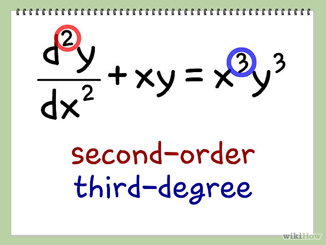
Order of differential equations

The order of a differential equation is determined by the highest derivative present in the equation. For example:

$\frac{d^3y}{dx^3} + \frac{d^2y}{dx^2} - y = 0$

This is a third-order equation because $\frac{d^3y}{dx^3}$ is the highest derivative that appears.

Why does order matter? It tells you how many initial conditions you need to pin down a unique solution:

• First-order equations need one initial condition: $y(x_0) = y_0$
• Second-order equations need two: $y(x_0) = y_0$ and $y'(x_0) = y'_0$
• Third-order equations need three: $y(x_0) = y_0$, $y'(x_0) = y'_0$, and $y''(x_0) = y''_0$

The pattern continues: an $n$th-order equation requires $n$ initial conditions.

Types of Differential Equations

Ordinary differential equations (ODEs) involve functions of a single independent variable and their derivatives. These are the focus of this unit. Partial differential equations (PDEs) involve functions of multiple independent variables and their partial derivatives; you won't encounter those in Calc II.

Within ODEs, you'll see several important subtypes:

• Separable equations can be rewritten so that all $x$-terms are on one side and all $y$-terms are on the other, letting you integrate each side independently. For instance, $\frac{dy}{dx} = xy$ can be separated into $\frac{1}{y}\,dy = x\,dx$.
• Linear equations have a specific form where the dependent variable and its derivatives appear only to the first power (no $y^2$, no $yy'$, etc.). A first-order linear ODE looks like $\frac{dy}{dx} + P(x)y = Q(x)$.
• Homogeneous linear equations are linear equations where $Q(x) = 0$, meaning every term involves the dependent variable or its derivatives.

Solutions to differential equations

A solution to a differential equation is any function that, when substituted into the equation, makes it true for all values of the independent variable in its domain. In other words, plugging the solution back in produces an identity.

Solutions can take different forms:

• Explicit: $y = f(x)$
• Implicit: $F(x, y) = 0$
• Parametric: $x = x(t)$, $y = y(t)$

Pay attention to the domain of your solution. For example, $y = \sqrt{1 - x^2}$ solves $\frac{dy}{dx} = -\frac{x}{\sqrt{1 - x^2}}$, but it's only valid for $-1 < x < 1$ (the endpoints make the derivative undefined). A solution that blows up or becomes imaginary outside some interval isn't wrong; it just has a restricted domain.

General vs particular solutions

The general solution represents the entire family of solutions to a differential equation. It contains arbitrary constants ($C_1$, $C_2$, etc.) that can take any value. The number of arbitrary constants matches the order of the equation.

For example, the general solution to $\frac{d^2y}{dx^2} + y = 0$ is:

$y = C_1\cos(x) + C_2\sin(x)$

Two constants, because it's a second-order equation.

A particular solution is what you get when you assign specific values to those constants, usually by applying initial or boundary conditions. If you're given $y(0) = 2$ and $y'(0) = -3$, you can solve for $C_1 = 2$ and $C_2 = -3$, giving the particular solution:

$y = 2\cos(x) - 3\sin(x)$

Think of it this way: the general solution is a whole family of curves, and the particular solution is the one specific curve that passes through the point and slope you've been given.

Initial-value problems and significance

An initial-value problem (IVP) pairs a differential equation with initial conditions that specify the value of the function (and possibly its derivatives) at a particular point, usually $x = 0$ or $t = 0$.

For example: solve $y' = y$ with $y(0) = 1$.

The general solution to $y' = y$ is $y = Ce^x$. Applying the initial condition: $y(0) = Ce^0 = C = 1$, so the particular solution is $y = e^x$.

The whole point of an IVP is to narrow down the infinite family of solutions to the one unique solution that fits your specific scenario. This is what makes differential equations useful in practice: you model the system with the equation, then use measured starting conditions to predict exactly what happens next.

Verification of differential equation solutions

Verification is a skill you'll use often, and it's more straightforward than solving. To check whether a function solves a differential equation:

1. Compute the necessary derivatives of the proposed solution
2. Substitute the function and its derivatives into the equation
3. Simplify and confirm that both sides are equal for all values of the independent variable

To verify a solution to an initial-value problem, add one more step:

1. Evaluate the function (and its derivatives, if needed) at the initial point and confirm the values match the given conditions

Example: Verify that $y = e^x$ solves $y' = y$ with $y(0) = 1$.

• Compute the derivative: $y' = e^x$
• Substitute into the equation: $e^x = e^x$ ✓ (true for all $x$)
• Check the initial condition: $y(0) = e^0 = 1$ ✓

Both checks pass, so $y = e^x$ is the verified solution. Get comfortable with this process; on exams, verification problems are essentially free points if you're careful with your algebra.