Definition of extreme value theory
Extreme value theory (EVT) is a branch of statistics focused on the behavior of extreme events and their probabilities. Rather than modeling the center of a distribution (like means or medians), EVT deals with the statistical behavior of the maximum or minimum of a set of random variables.
EVT provides a framework for estimating the likelihood of rare events that fall outside the range of typical observations. Think of it this way: standard statistical tools describe what usually happens, while EVT describes what happens in the worst case.
Importance in actuarial science
Actuaries use EVT to assess and manage risks tied to extreme events such as natural disasters and financial market crashes. Without EVT, pricing insurance products and setting adequate reserves for catastrophic losses would rely on guesswork about the tails of the distribution.
EVT enables actuaries to estimate both the probability and magnitude of extreme losses. This is directly tied to solvency requirements: regulators need to know that an insurer can survive a 1-in-200-year event, and EVT gives you the tools to quantify what that event looks like.
Types of extreme value distributions
Gumbel distribution
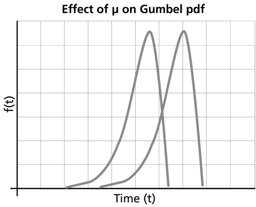
The Gumbel distribution (Type I extreme value distribution) models the distribution of the maximum or minimum of a large number of independent and identically distributed random variables. It's the limiting distribution when the underlying data has exponentially decaying tails (like normal or exponential distributions).
- CDF: , where is the location parameter and is the scale parameter
- The tails are "light" relative to the other extreme value types
- Common applications: flood level modeling in hydrology, extreme market movements in finance
Fréchet distribution
The Fréchet distribution (Type II extreme value distribution) models the maximum of random variables with heavy tails. This is the one you'll encounter most often in actuarial loss modeling, because insurance losses tend to be heavy-tailed.
- CDF: for , where is the location parameter, is the scale parameter, and is the shape parameter
- The shape parameter controls how heavy the tail is: smaller means a heavier tail
- Common applications: extreme financial losses, material strength in engineering
Weibull distribution (as extreme value type)
The Weibull distribution (Type III extreme value distribution) models the minimum of random variables with bounded (light) tails. Note that this is the Weibull in its role as an extreme value distribution, which is distinct from its more general use in reliability.
- CDF: for , where is the location parameter, is the scale parameter, and is the shape parameter
- The distribution has a finite upper endpoint, making it appropriate when there's a natural bound on the variable
- Common applications: component failure times in reliability engineering, wind speed modeling
Generalized extreme value distribution
The generalized extreme value (GEV) distribution unifies all three types into a single parametric form. Instead of deciding which type to use upfront, you fit the GEV and let the shape parameter tell you which type the data supports.
- CDF: for
- Parameters: (location), (scale), (shape)
The shape parameter determines the tail type:
| value | Distribution type | Tail behavior |
|---|---|---|
| Gumbel | Light-tailed (exponential decay) | |
| Fréchet | Heavy-tailed (polynomial decay) | |
| Weibull | Bounded upper tail |
For actuarial loss modeling, is the most common and most dangerous case.
Fisher-Tippett-Gnedenko theorem
This theorem is the theoretical backbone of EVT. It states that the properly normalized maximum of a large number of i.i.d. random variables converges in distribution to one of the three extreme value types (Gumbel, Fréchet, or Weibull).
This is analogous to the Central Limit Theorem, but for maxima instead of sums. Just as the CLT justifies using the normal distribution for sample means regardless of the underlying distribution, the Fisher-Tippett-Gnedenko theorem justifies using extreme value distributions for sample maxima.
Which of the three types you converge to depends on the tail behavior of the underlying distribution. Heavy-tailed parent distributions lead to Fréchet; light-tailed ones lead to Gumbel; bounded distributions lead to Weibull.
Block maxima method
The block maxima method is one of two main approaches for applying EVT to data. Here's how it works:
- Divide your time series into non-overlapping blocks of equal size (e.g., annual blocks for daily data).
- Extract the maximum value from each block.
- Fit a GEV distribution to the resulting set of block maxima.
- Use the fitted GEV to estimate return levels and tail probabilities.
The choice of block size involves a tradeoff. Blocks that are too small introduce bias because the asymptotic approximation hasn't kicked in yet. Blocks that are too large leave you with very few maxima to estimate parameters from. Annual blocks are the most common choice in practice, balancing these concerns.
Peaks over threshold method
The peaks over threshold (POT) method is an alternative that often makes better use of the data. Instead of taking only one value per block, it uses all observations that exceed a high threshold.
-
Choose a high threshold .
-
Extract all observations that exceed .
-
Model the exceedances using a generalized Pareto distribution (GPD).
-
Use the fitted GPD to estimate tail probabilities and return levels.
Choosing the threshold is the key practical challenge. Too low, and the GPD approximation is poor. Too high, and you have too few exceedances for reliable estimation. Two common tools for threshold selection:
- Mean excess plot: Plot the mean of exceedances against the threshold. The GPD assumption implies this should be approximately linear above the correct threshold.
- Threshold stability plot: Fit the GPD at a range of thresholds and look for the region where the shape parameter estimate stabilizes.
The POT method is generally more data-efficient than block maxima because it uses all extreme observations, not just one per block.
Generalized Pareto distribution
The generalized Pareto distribution (GPD) models the distribution of excesses over a high threshold. It's the natural companion to the GEV: the GEV models block maxima, while the GPD models threshold exceedances.
- CDF: for and
- Parameters: (scale), (shape)
The shape parameter controls the tail:
- : Exponential tail (light-tailed)
- : Heavy-tailed (Pareto-like, polynomial decay)
- : Bounded upper tail (finite endpoint at )
The GPD shape parameter is the same as the GEV shape parameter when both are applied to the same underlying process. This connection is theoretically grounded and practically useful.
Estimating parameters of extreme value distributions
Maximum likelihood estimation
Maximum likelihood estimation (MLE) maximizes the likelihood function to find parameter estimates. It's the most widely used method for GEV and GPD fitting.
- Provides asymptotically efficient and consistent estimates under regularity conditions
- Can be computationally intensive for large datasets
- One caveat: for the GEV with , the regularity conditions for MLE break down, and the method may not perform well
Probability weighted moments
Probability weighted moments (PWMs) are based on the moments of the order statistics.
- Computationally simpler than MLE
- Performs well for small to moderate sample sizes
- May be less efficient than MLE for large samples
L-moments
L-moments are linear combinations of probability weighted moments and tend to be more robust.
- Less sensitive to outliers than conventional moments or MLE
- Good small-sample properties
- Less sensitive to threshold choice in the POT method
- May be less efficient than MLE when the sample is large and the model is correctly specified
In practice, comparing estimates across methods is a useful diagnostic. If MLE and L-moment estimates disagree substantially, that's a signal to investigate further.
Return level estimation
The return level is the value expected to be exceeded on average once every periods. For example, the 100-year return level for flood losses is the loss amount you'd expect to be exceeded once every 100 years on average.
To estimate a return level:
- Fit a GEV (block maxima) or GPD (peaks over threshold) to your extreme data.
- Invert the fitted CDF to find the quantile corresponding to the desired exceedance probability .
- For the GEV, the -year return level is:
Uncertainty in return level estimates grows rapidly as increases. A 1000-year return level has much wider confidence intervals than a 10-year return level. Confidence intervals can be constructed using profile likelihood, delta method, or bootstrap approaches.
Definition of heavy-tailed distributions
A distribution is heavy-tailed if its tails decay slower than any exponential distribution. Formally, a distribution is heavy-tailed if:
Equivalently, the moment generating function is infinite for all .
The practical implication: heavy-tailed distributions assign meaningfully higher probability to extreme values than distributions like the normal or exponential. A single extreme observation can dominate the sum of all other observations.
Properties of heavy-tailed distributions
- Slowly decaying tails: The probability of very large values decreases much more slowly than in light-tailed distributions. For a Pareto distribution with , the probability of exceeding 10 times the minimum is , while for an exponential distribution it would be negligibly small.
- Potentially infinite moments: Depending on how heavy the tail is, some or all moments may be infinite. The Cauchy distribution has no finite moments at all. A Pareto with has a finite mean and variance but infinite third moment.
- Concentration of risk: A large portion of the total loss can come from a small number of extreme events. This is sometimes called the "catastrophe property."
- Greater estimation uncertainty: Sample statistics like the mean and variance converge more slowly, making parameter estimation harder and less stable.
Examples of heavy-tailed distributions
![Gumbel distribution, Distributions [HDip Data Analytics]](https://storage.googleapis.com/static.prod.fiveable.me/search-images%2F%22Gumbel_distribution_extreme_value_theory_CDF_flood_levels_finance_maximum_minimum_random_variables%22-gumbel_distribution.png%3Fw%3D200%26tok%3D2a61f2.png)
Pareto distribution
The Pareto distribution is the canonical heavy-tailed distribution and follows a power law. It's widely used to model insurance losses, income distributions, and city populations.
- PDF: for , where is the minimum value and is the shape (tail index) parameter
- The tail probability decays as a power law:
- Smaller means heavier tails. With , the mean is infinite. With , the mean exists but the variance is infinite.
Log-normal distribution
A random variable is log-normally distributed if its natural logarithm is normally distributed. The log-normal is heavy-tailed, though less extreme than the Pareto.
- PDF: for
- and are the mean and standard deviation of , not of itself
- All moments are finite, but the tail is still heavier than exponential
- The tail heaviness increases with . For large , the log-normal can look very similar to a Pareto in practice.
- Common in modeling aggregate insurance losses and financial asset prices
Weibull distribution with shape parameter < 1
When the Weibull shape parameter , the distribution becomes heavy-tailed (technically, it's "subexponential" but not regularly varying like the Pareto).
- PDF: for
- implies a decreasing hazard rate: the longer a component has survived, the less likely it is to fail soon
- Used in reliability engineering and certain insurance applications
Comparison of heavy-tailed vs light-tailed distributions
| Property | Light-tailed (Normal, Exponential) | Heavy-tailed (Pareto, Log-normal) |
|---|---|---|
| Tail decay | Exponential or faster | Slower than exponential |
| Extreme event probability | Very low | Meaningfully higher |
| Moments | All finite | May be infinite |
| MGF | Finite in a neighborhood of 0 | Infinite for all |
| Parameter estimation | Relatively stable | Sensitive to extreme observations |
| Risk of underestimation | Low | High if wrong model assumed |
The single most important takeaway: if you fit a light-tailed model to data that's actually heavy-tailed, you will systematically underestimate the probability and severity of extreme losses.
Implications of heavy-tailed distributions in risk management
Heavy tails have direct consequences for actuarial practice:
- VaR underestimation: Value-at-Risk computed under normal or other light-tailed assumptions can dramatically underestimate the true risk. A 99.5th percentile loss under a Pareto model can be many times larger than under a normal model with the same mean and variance.
- Capital adequacy: Regulators (e.g., under Solvency II) require capital to cover extreme losses. Using the wrong distributional assumption can lead to inadequate reserves.
- Dependence amplification: When multiple heavy-tailed risks are dependent, the joint tail risk can be much worse than the sum of individual tail risks. This is where copulas become essential.
- Reinsurance pricing: Reinsurance covers the tail of the loss distribution. Getting the tail shape wrong directly translates to mispriced reinsurance contracts.
Modeling extreme events with heavy-tailed distributions
EVT and heavy-tailed distributions come together in practice through the POT approach:
- Identify that your loss data is heavy-tailed (using diagnostic tools like QQ plots, mean excess plots, or Hill plots).
- Choose an appropriate threshold using the mean excess plot (should be approximately linear above the correct threshold) or threshold stability plots.
- Fit a GPD to the exceedances above .
- Use the fitted GPD to compute tail probabilities, return levels, and risk measures (VaR, TVaR).
- Assess goodness-of-fit using tests like Anderson-Darling or Kolmogorov-Smirnov, along with PP and QQ plots.
The mean excess function is a particularly useful diagnostic. For a Pareto distribution, is linear and increasing in . For an exponential distribution, is constant. If your data's mean excess plot is increasing, that's strong evidence of heavy tails.
Challenges in estimating parameters of heavy-tailed distributions
- High variance of estimates: Extreme observations have outsized influence on parameter estimates, leading to instability, especially with small samples.
- Method sensitivity: MLE, PWM, and L-moments can give noticeably different results for the same dataset. It's good practice to compare methods and understand why they differ.
- Threshold selection: In the POT method, results can be sensitive to the threshold choice. There's no universally "correct" threshold, so sensitivity analysis across a range of thresholds is standard practice.
- Covariates: When loss severity depends on explanatory variables (e.g., geographic location, policy type), you need regression models for the GPD parameters, which adds complexity.
- Model uncertainty: You can never be certain you've chosen the right distributional family. Techniques like model averaging, Bayesian model comparison, or fitting multiple candidate distributions and comparing via information criteria (AIC, BIC) help address this.
Importance of tail risk in actuarial applications
Tail risk is the risk of losses in the extreme tail of the distribution. For actuaries, getting tail risk right is a balancing act:
- Underestimation leads to insufficient reserves and capital, potentially causing insolvency after a catastrophic event.
- Overestimation leads to excessive premiums and capital charges, making the company uncompetitive.
Effective tail risk management combines several elements:
- Robust statistical models (EVT, heavy-tailed distributions)
- Stress testing and scenario analysis for events beyond the model's range
- Risk transfer mechanisms (reinsurance, catastrophe bonds, hedging)
- Regular model validation and backtesting against emerging experience
Copulas for modeling dependence in extreme events
Copulas are functions that link marginal distributions to form a joint distribution, separating the dependence structure from the individual risk profiles. They're essential when modeling multiple heavy-tailed risks together.
Why copulas matter for extremes: standard correlation (Pearson's) doesn't capture tail dependence. Two risks can have moderate overall correlation but very high dependence in extreme scenarios (e.g., multiple lines of business all hit by the same hurricane).
Key copula families and their tail dependence properties:
- Gaussian copula: No tail dependence (even if correlation is high, joint extremes are asymptotically independent). This was a major issue in the 2008 financial crisis.
- Student-t copula: Symmetric tail dependence in both tails. The degree of tail dependence increases as the degrees of freedom decrease.
- Archimedean copulas (Clayton, Gumbel, Frank): Can model asymmetric dependence. Clayton captures lower tail dependence; Gumbel captures upper tail dependence.
Copula parameter estimation with limited extreme data is challenging. Bayesian methods or expert judgment may be needed to supplement the data, especially for joint tail behavior where observations are scarce.