Aggregate Loss Distributions
Aggregate loss distributions model the total losses an insurance company incurs over a defined period. By combining a frequency distribution (how many claims occur) with a severity distribution (how large each claim is), actuaries can estimate the full range of possible total losses. These models are foundational for setting premiums, establishing reserves, and structuring reinsurance.
Stop-loss reinsurance builds directly on these models. It protects insurers against aggregate losses that exceed a specified threshold, transferring tail risk to a reinsurer. Understanding both the aggregate loss distribution and the mechanics of stop-loss coverage is essential for managing catastrophic or unexpectedly large losses.
Aggregate Loss Distributions
An aggregate loss represents the total claims paid over a specific period (a policy term, quarter, or year). It's defined as:
where is the random number of claims (frequency) and is the size of the -th claim (severity). The three building blocks are the frequency distribution, the severity distribution, and the compound model that ties them together.
Models of Aggregate Losses
Aggregate loss models combine a frequency distribution for with a severity distribution for each to produce the distribution of . The most common compound models are:
- Compound Poisson — the default starting point; assumes claims arrive independently at a constant rate
- Compound negative binomial — used when claim counts show overdispersion (variance exceeds the mean)
- Compound binomial — used when there's a fixed, known number of exposure units
Selecting the right model depends on the characteristics of the risk. Actuaries rely on historical data, goodness-of-fit tests, industry benchmarks, and expert judgment to choose.
Frequency Distributions
Frequency distributions describe the probability of observing a specific number of claims in a given period. The three standard choices each suit different situations:
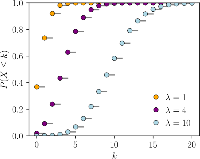
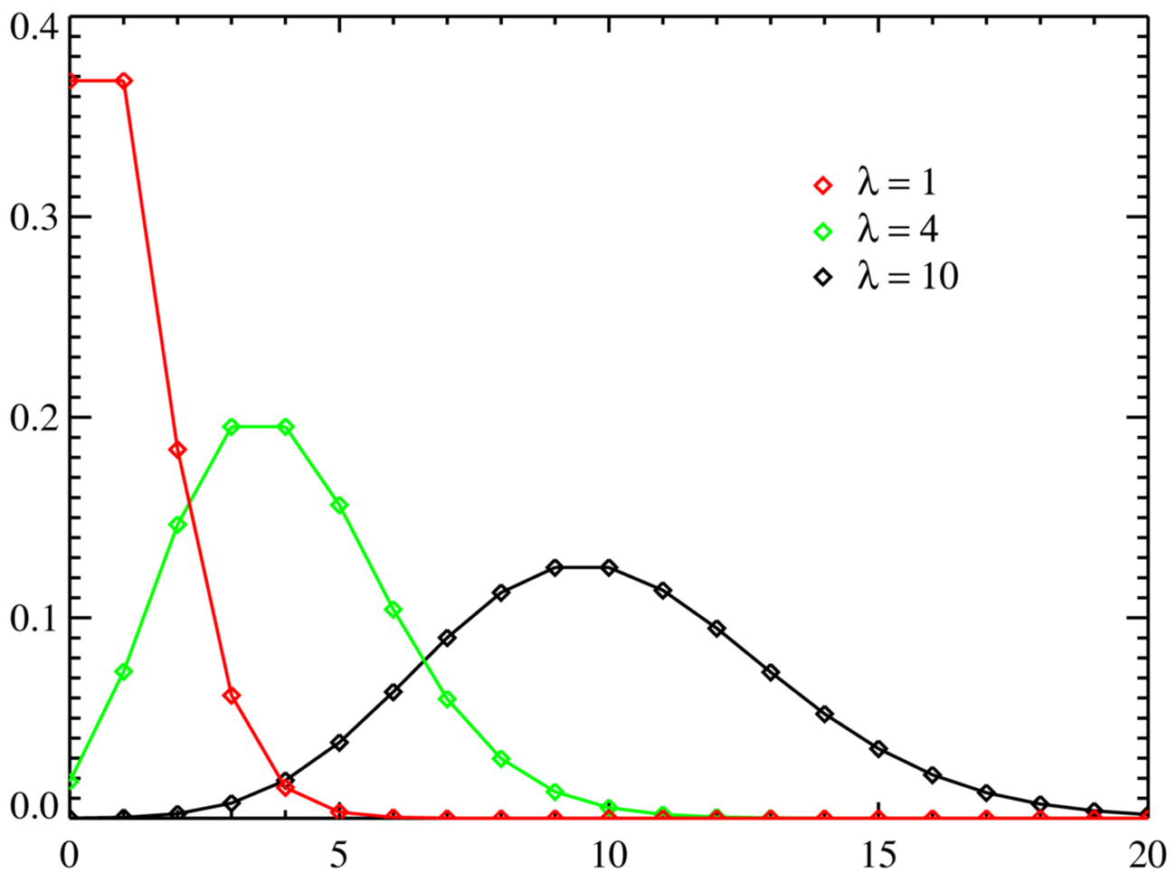
- Poisson — Claims occur independently at a constant average rate . The mean equals the variance (). Commonly applied in auto insurance where individual claim events are roughly independent.
- Negative binomial — Appropriate when there is overdispersion, meaning . This often arises in health insurance, where unobserved heterogeneity among insureds causes extra variability in claim counts.
- Binomial — Used when there is a fixed number of exposure units , each with the same claim probability . Typical in group life insurance where you know exactly how many lives are covered.
Severity Distributions
Severity distributions model the size or cost of individual claims. Common choices include:
- Lognormal — Works well for claims that are mostly moderate but occasionally very large (property damage)
- Gamma — Flexible shape; often used for medical claims
- Pareto — Heavy-tailed; suited for liability or catastrophe claims where extreme values are more likely
- Weibull — Useful when the hazard rate changes over time
Actuaries assess fit using goodness-of-fit tests (Kolmogorov-Smirnov, Anderson-Darling, chi-square) and graphical tools like Q-Q plots and histograms overlaid with the fitted density.
Compound Poisson Distribution
The compound Poisson model assumes and the are i.i.d. with common distribution. Its key moments have clean formulas:
That variance formula is worth memorizing. Notice it uses the second raw moment , not the variance of . This follows from the law of total variance.
The compound Poisson model also has a useful additivity property: if two independent portfolios each follow compound Poisson distributions, their combined aggregate loss is also compound Poisson. This makes it convenient for merging books of business.
Compound Negative Binomial Distribution
When claim count data shows overdispersion, the compound negative binomial is a better fit. Here with and .
The moments of are:
This second term, , captures the extra variability from the overdispersed claim count. Compared to the compound Poisson, aggregate losses will have a heavier right tail.
Compound Binomial Distribution
The compound binomial model applies when there are exactly exposure units, each independently generating a claim with probability . So .
This model is less commonly used than the other two because most real portfolios don't have a strict fixed number of independent units. However, it's natural for group coverages where the roster is known. Its PMF can be computed via convolutions or recursive methods.
Convolutions vs. Recursive Methods
Once you've chosen frequency and severity distributions, you need to actually compute the distribution of . Two main approaches exist:
Convolutions compute the distribution of by directly combining the severity distribution with itself, weighted by the frequency probabilities. For a discrete severity with possible values , the -fold convolution gives the distribution of the sum of claims. This is conceptually straightforward but computationally expensive for large portfolios.
Panjer's recursion is far more efficient. It applies when the frequency distribution belongs to the class, meaning:
The Poisson, negative binomial, and binomial distributions all satisfy this condition. The recursive formula for the aggregate loss probabilities (with discrete severity) is:
Starting from , you build up the entire distribution of iteratively. This is much faster than computing convolutions directly.
Aggregate Claims Examples
Example 1 (Compound Poisson): An auto insurer expects an average of claims per policy year. Claim sizes follow a lognormal distribution with mean $5,000 and standard deviation $2,000.
- To find , you need
- , so
Example 2 (Compound Negative Binomial): A health insurer observes and (overdispersion ratio of 2). Claim sizes follow a gamma distribution with mean $2,000 and standard deviation $1,000.
Notice how the overdispersion in claim counts dramatically increases the variance of aggregate losses compared to what a Poisson model would give (which would yield ).
Stop-Loss Reinsurance
Reinsurance allows an insurer to transfer part of its risk to another company (the reinsurer). Stop-loss reinsurance specifically covers aggregate losses that exceed a chosen threshold (the retention) over a defined period. The reinsurer pays , and the insurer keeps everything up to .
Purpose of Reinsurance
Reinsurance serves several functions:
- Volatility reduction — Smooths financial results by capping the insurer's worst-case losses
- Capacity expansion — With less risk retained, the insurer can underwrite more business
- Diversification — Transfers concentrated risk to reinsurers who pool it across many cedants and geographies
- Capital management — Helps meet regulatory capital requirements (e.g., risk-based capital) and maintain credit ratings
Types of Reinsurance
The two broad categories are:
- Treaty reinsurance — Covers an entire portfolio of risks under a long-term agreement. The reinsurer must accept all risks that fall within the treaty's terms.
- Facultative reinsurance — Covers a specific individual risk or policy, negotiated case by case. Used for unusual or very large exposures.
Within each category, reinsurance can be structured as:
- Proportional — The reinsurer takes a fixed share of premiums and losses. Includes quota share (fixed percentage of every policy) and surplus share (reinsurer covers amounts above a line retained by the insurer).
- Non-proportional — The reinsurer pays only when losses exceed a threshold. Includes excess of loss (per-claim basis) and stop-loss (aggregate basis).
Excess of Loss vs. Stop-Loss
These are both non-proportional, but they trigger differently:
| Feature | Excess of Loss | Stop-Loss |
|---|---|---|
| Trigger | Individual claim exceeds retention | Aggregate losses exceed retention |
| Reinsurer pays | per claim | for total losses |
| Common use | Property and casualty | Health and life |
| Protects against | Single large claims | Accumulation of many claims |
Stop-loss reinsurance can be further divided into individual stop-loss (ISL), which caps losses on any single covered member, and aggregate stop-loss (ASL), which caps total losses across the entire group.
Determining Stop-Loss Premiums
The net stop-loss premium (also called the pure premium) is the expected value of the reinsurer's payout:
This can also be written as:
where .
To compute this in practice:
-
Model the aggregate loss distribution using the appropriate compound model
-
Calculate and from the distribution
-
Add a risk margin (loading) to reflect the reinsurer's cost of capital and parameter uncertainty
-
The gross stop-loss premium is , where is the loading factor
The loading factor varies by reinsurer and depends on the tail risk, the cedant's loss history, and market conditions.
Impact on Aggregate Losses
Stop-loss reinsurance transforms the insurer's retained loss from to . This has several effects on the distribution:
- The right tail is truncated at . The insurer's maximum possible loss becomes .
- The variance decreases because extreme outcomes are removed.
- The mean retained loss drops from to .
Actuaries must account for this truncation when pricing the underlying insurance policies and when calculating reserves. Ignoring the reinsurance would overstate the insurer's risk; ignoring the reinsurance cost would understate expenses.
Advantages of Stop-Loss
- Protects against catastrophic accumulations of losses that could threaten solvency
- Reduces earnings volatility, making financial results more predictable
- Frees up capital that can be deployed to write additional business
- Helps satisfy regulatory solvency requirements
Disadvantages of Stop-Loss
- Cost — Premiums can be substantial, especially for low retentions or volatile portfolios
- Basis risk — The reinsurance terms may not perfectly align with the insurer's actual loss experience (e.g., different definitions of covered losses)
- Moral hazard — With downside protection in place, insurers may relax underwriting discipline or take on riskier business
- Reinsurer restrictions — Reinsurers may impose exclusions, caps, or strict underwriting guidelines that limit the insurer's flexibility
Optimal Stop-Loss Retention
Choosing the retention is a balancing act. A lower gives more protection but costs more in reinsurance premium. A higher is cheaper but leaves the insurer exposed to larger aggregate losses.
Actuaries determine the optimal retention by:
- Modeling the aggregate loss distribution under various retention levels
- Computing risk measures for the retained loss at each level, such as Value-at-Risk (VaR) at a chosen confidence level or Conditional Tail Expectation (CTE) (also called TVaR)
- Comparing the marginal reduction in risk against the marginal increase in reinsurance cost
- Selecting the retention that minimizes a chosen objective function (e.g., total cost of risk = retained losses + reinsurance premium + cost of capital)
The optimal depends on the insurer's risk appetite, available capital, the portfolio's loss characteristics, and the reinsurer's pricing. The reinsurer's financial strength and claims-paying reputation also matter, since the insurer is relying on the reinsurer to pay when losses are at their worst.