3.2 Annuities and perpetuities

Annuities and perpetuities are structured payment streams that form the backbone of financial mathematics. Mastering their valuation is essential for pricing insurance products, designing pension plans, analyzing bonds, and working with any contract that involves a series of cash flows over time.

Types of annuities

An annuity is a financial contract that provides a series of payments over a specified period. Before diving into formulas, you need to understand the classification system, since the type of annuity determines which formula applies.

Ordinary vs due

• Ordinary annuities have payments made at the end of each period (end of month, quarter, or year).
• Annuities due have payments made at the beginning of each period.

The timing difference matters more than it might seem. Because annuity-due payments arrive one period earlier, each payment has one less period of discounting. This makes an annuity due always worth more than an otherwise identical ordinary annuity by a factor of $(1+i)$.

Certain vs contingent

• Annuities-certain have a fixed number of guaranteed payments regardless of any external event.
• Contingent annuities have payments that depend on some event occurring, most commonly the survival or death of an individual (life annuities).

For contingent annuities, you must incorporate the probability of the triggering event into the valuation. This unit focuses on annuities-certain; contingent annuities appear in life contingencies.

Level vs varying

• Level annuities pay the same amount every period.
• Varying annuities have payments that change over time: increasing by a fixed amount (arithmetic), increasing by a percentage (geometric), or following some other pattern.

Varying annuities require more complex calculations because you can't simply factor out a single payment amount. You'll often need to work with increasing annuity symbols like $(Ia)_{\overline{n}|}$ or $(Da)_{\overline{n}|}$.

Temporary vs perpetuity

• Temporary annuities run for a fixed term with a limited number of payments (e.g., 5-year, 10-year, or 20-year).
• Perpetuities continue forever with an infinite number of payments.

Perpetuities are simpler to value than you might expect, since the infinite geometric series converges to a clean formula (covered below).

Annuity-certain valuation

Annuity-certain valuation involves calculating the present value and accumulated value of annuities with guaranteed payments. These calculations are foundational for pricing and reserving.

Present value of annuity-certain

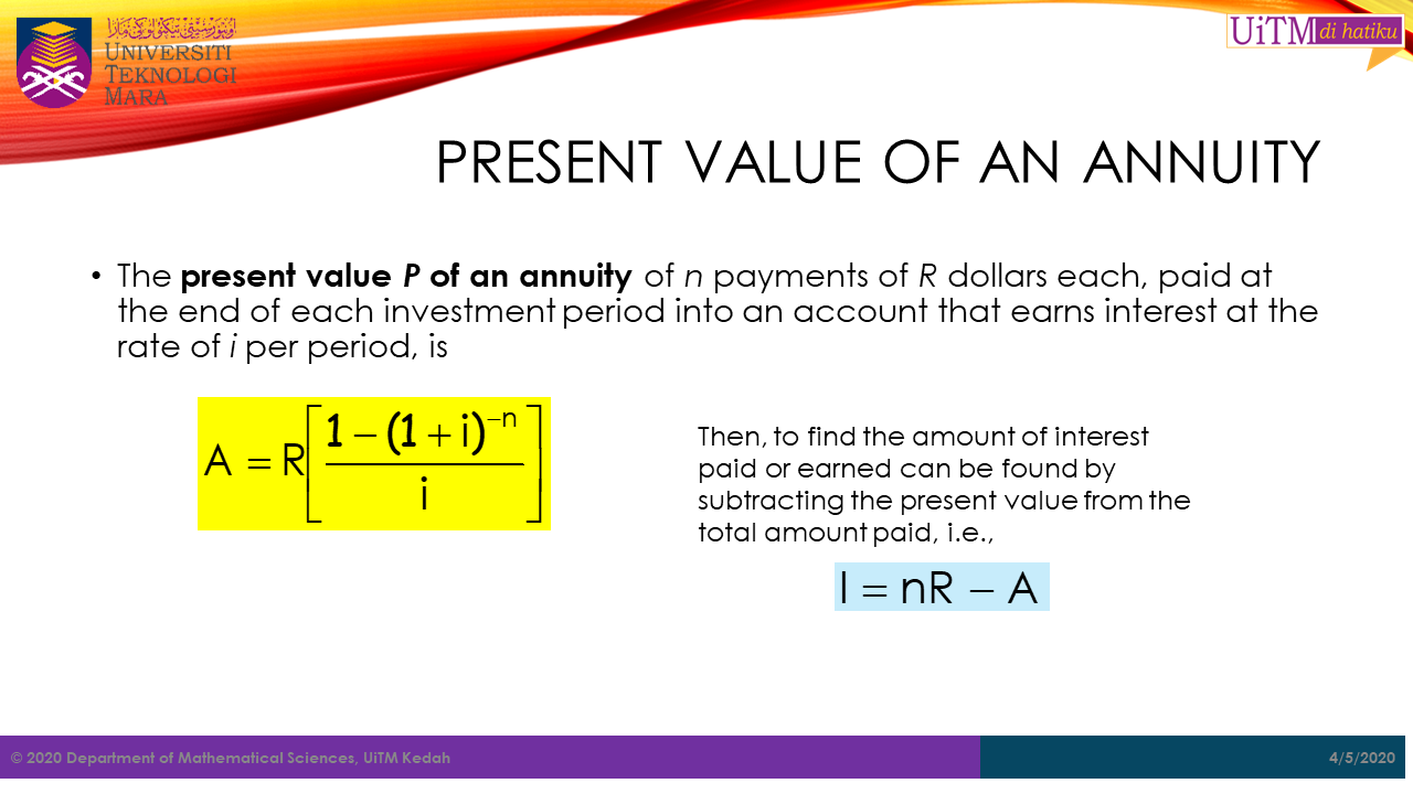
The present value of an annuity-certain is the lump sum today that's equivalent to the entire stream of future payments at a given interest rate. You're summing up each payment discounted back to time zero.

For an ordinary annuity-certain paying 1 per period for $n$ periods:

$a_{\overline{n}|} = \frac{1-v^n}{i}$

where $v = \frac{1}{1+i}$ is the discount factor and $i$ is the effective interest rate per period.

To build intuition: each of the $n$ payments of 1 is worth $v^t$ at time zero (where $t$ is the time of payment). Summing the geometric series $v + v^2 + \cdots + v^n$ gives you the formula above.

Accumulation of annuity-certain

The accumulated value (future value) is the total amount you'd have at the end of the annuity term if all payments were invested at rate $i$.

$s_{\overline{n}|} = \frac{(1+i)^n - 1}{i}$

Notice the relationship: $s_{\overline{n}|} = a_{\overline{n}|} \cdot (1+i)^n$. The accumulated value is just the present value carried forward $n$ periods.

Annuity-certain with non-level payments

When payment amounts vary, you can't use the standard annuity symbol directly. Common approaches:

• Sum individual payments: Calculate $\sum_{t=1}^{n} P_t \cdot v^t$ where $P_t$ is the payment at time $t$.
• Arithmetic increases: If payments increase by a fixed amount each period, use the increasing annuity $(Ia)_{\overline{n}|}$ or decreasing annuity $(Da)_{\overline{n}|}$ formulas.
• Geometric increases: If payments grow at rate $g$ per period, the present value becomes a modified geometric series that can be evaluated in closed form (provided $g \neq i$).

Annuity-certain with payments in advance

For an annuity due, payments arrive at the beginning of each period. The formulas relate directly to the ordinary annuity:

$\ddot{a}_{\overline{n}|} = (1+i) \cdot a_{\overline{n}|} = \frac{1 - v^n}{d}$

$\ddot{s}_{\overline{n}|} = (1+i) \cdot s_{\overline{n}|}$

Here $d = \frac{i}{1+i}$ is the discount rate. The $(1+i)$ multiplier reflects that every payment is received one period sooner, so each is worth $(1+i)$ times more.

Annuities payable continuously

Continuously paid annuities model situations where payments flow as a constant stream rather than arriving at discrete intervals. While no real payment is truly continuous, this is a useful theoretical tool and a good approximation for very frequent payments.

Present value of continuous annuity

The present value is found by integrating the discounted payment stream over the term:

$\bar{a}_{\overline{n}|} = \int_0^n e^{-\delta t} \, dt = \frac{1 - e^{-\delta n}}{\delta}$

where $\delta$ is the force of interest (the continuously compounded rate).

Accumulation of continuous annuity

$\bar{s}_{\overline{n}|} = \frac{e^{\delta n} - 1}{\delta}$

As with discrete annuities, $\bar{s}_{\overline{n}|} = \bar{a}_{\overline{n}|} \cdot e^{\delta n}$.

Relationship between discrete and continuous annuities

The force of interest $\delta$ connects to the effective annual rate $i$ through:

$\delta = \ln(1+i)$

As you increase the payment frequency of a discrete annuity (monthly → weekly → daily → ...), its present value converges to the continuous annuity value. This means $\bar{a}_{\overline{n}|}$ is the limiting case of $a_{\overline{n}|}^{(m)}$ as $m \to \infty$.

Perpetuities

A perpetuity pays forever. Because the payments never stop, you might expect the present value to be infinite, but as long as the interest rate is positive, the discounted payments form a convergent geometric series.

Present value of perpetuity

For a level ordinary perpetuity paying 1 per period:

$a_{\overline{\infty}|} = \frac{1}{i}$

This follows directly from the annuity formula by taking $\lim_{n \to \infty} \frac{1 - v^n}{i}$. Since $0 < v < 1$, the $v^n$ term vanishes, leaving $\frac{1}{i}$.

At $i = 5\%$, a perpetuity of 1 per year has a present value of $\frac{1}{0.05} = 20$.

Perpetuity with non-level payments

For a perpetuity whose payments increase by a fixed amount $g$ each period (so payments are $1, 1+g, 1+2g, \ldots$), the present value is:

$PV = \frac{1}{i} + \frac{g}{i^2}$

For a perpetuity with payments growing at a constant rate $r$ per period (geometric growth), the present value is:

$PV = \frac{1}{i - r} \quad \text{(valid only when } i > r\text{)}$

Be careful to distinguish between arithmetic increases (fixed dollar amount $g$) and geometric increases (fixed rate $r$).

Perpetuity with payments in advance

A perpetuity due pays at the beginning of each period. Its present value is:

$\ddot{a}_{\overline{\infty}|} = \frac{1+i}{i} = \frac{1}{d}$

where $d = \frac{i}{1+i}$ is the discount rate. This is $(1+i)$ times the ordinary perpetuity value, following the same pattern as finite annuities.

Relationship between annuities and perpetuities

A perpetuity is the limiting case of a temporary annuity as $n \to \infty$. You can also decompose a perpetuity into pieces:

$a_{\overline{\infty}|} = a_{\overline{n}|} + v^n \cdot a_{\overline{\infty}|}$

This says a perpetuity equals an $n$-year annuity plus a deferred perpetuity starting at time $n$. Rearranging gives you the standard annuity formula, which is a useful way to verify your work.

Annuities payable more frequently than interest convertible

When payments occur $m$ times per year but interest is quoted as an annual effective rate, you need to adjust the formulas to account for the mismatch.

Present value of annuity payable m-thly

An annuity paying $\frac{1}{m}$ at the end of each $m$-th of a year (so that the total annual payment is 1) for $n$ years has present value:

$a_{\overline{n}|}^{(m)} = \frac{1 - v^n}{i^{(m)}}$

where $i^{(m)}$ is the nominal annual interest rate compounded $m$ times per year, defined by:

$(1 + \tfrac{i^{(m)}}{m})^m = 1 + i$

So $i^{(m)} = m\left[(1+i)^{1/m} - 1\right]$. Note that $i^{(m)}$ is not simply $\frac{i}{m}$; that common mistake will cost you on exams.

Accumulation of annuity payable m-thly

$s_{\overline{n}|}^{(m)} = \frac{(1+i)^n - 1}{i^{(m)}}$

The relationship $s_{\overline{n}|}^{(m)} = a_{\overline{n}|}^{(m)} \cdot (1+i)^n$ still holds.

Valuation of annuities payable p-thly

When payments are made $p$ times per year and interest is compounded $m$ times per year, the approach is the same: convert everything to a common basis. Find the effective rate per payment period and apply the standard annuity formula with the appropriate number of total payment periods and the effective rate per period.

The key principle is: match the interest rate to the payment period. If payments are monthly, you need the effective monthly rate. If payments are quarterly, you need the effective quarterly rate.

Solving for unknown parameters

In practice, you'll often know some parameters and need to find others. The annuity formulas can be rearranged to solve for the payment amount, interest rate, or term.

Solving for payment amount

Given the present value $PV$, interest rate $i$, and term $n$, the level payment $P$ for an ordinary annuity-certain is:

$P = \frac{PV}{a_{\overline{n}|}} = \frac{PV \cdot i}{1 - v^n}$

This is exactly what happens when a bank calculates your mortgage payment.

Solving for interest rate

Finding $i$ when you know $PV$, $P$, and $n$ requires solving:

$PV = P \cdot \frac{1 - (1+i)^{-n}}{i}$

This equation has no closed-form solution for $i$. You'll need to use:

1. Numerical methods such as Newton-Raphson or bisection
2. Linear interpolation between two trial rates that bracket the answer
3. Calculator/spreadsheet functions like RATE (Excel) or IRR

On exams, you'll typically use interpolation or be given enough information to avoid a full numerical solve.

Solving for term of annuity

Given $PV$, $P$, and $i$, solve for $n$:

1. Start with $PV = P \cdot \frac{1 - v^n}{i}$

2. Rearrange: $v^n = 1 - \frac{PV \cdot i}{P}$

3. Take logarithms: $n = \frac{\ln\left(1 - \frac{PV \cdot i}{P}\right)}{\ln(v)}$

where $v = \frac{1}{1+i}$.

Watch for the case where $\frac{PV \cdot i}{P} \geq 1$. This means the payment $P$ isn't large enough to ever pay off the present value at rate $i$, so no finite $n$ exists. Also note that $n$ may not be a whole number, which means the final payment will typically be a smaller "drop payment" or a slightly larger "balloon payment."

Applications of annuities and perpetuities

Loans and mortgages

A standard amortizing loan is an ordinary annuity-certain. The borrower receives the present value (loan principal) and makes level payments that cover both interest and principal repayment. Using the annuity payment formula, you can calculate the periodic payment, and from there build a full amortization schedule showing how much of each payment goes to interest vs. principal.

Pension plans and retirement income

Pension plans use annuity valuation to determine how much money must be set aside today to fund future retirement payments. A defined-benefit pension promising $P$ per month for life is valued as a life annuity (contingent), but the financial mathematics portion uses annuity-certain techniques as the starting point. Converting a lump-sum retirement balance into a steady income stream is a direct application of solving for the payment amount.

Bonds and fixed-income securities

A bond's price equals the present value of its future cash flows. The coupon payments form an annuity, and the face value repayment at maturity is a single lump sum:

$\text{Bond Price} = C \cdot a_{\overline{n}|} + F \cdot v^n$

where $C$ is the coupon payment, $F$ is the face value, and $n$ is the number of periods to maturity. A consol (perpetual bond) with no maturity date is valued as a perpetuity: $\text{Price} = \frac{C}{i}$.

Leases and rental agreements

Lease payments form an annuity (often an annuity due, since rent is typically paid at the start of each period). Comparing the present value of lease payments against the purchase price of an asset helps determine whether leasing or buying is more cost-effective. The same annuity formulas apply, with attention to whether payments are in advance or in arrears.