5.2 Compound Poisson processes and claim frequency

Compound Poisson processes are key in actuarial math, modeling claim frequency and severity over time. They combine Poisson processes for event frequency with separate distributions for event magnitude, providing a framework for analyzing aggregate losses in insurance.

This topic explores the fundamentals, applications, and modifications of compound Poisson processes. It covers parameter estimation, simulation techniques, and generalizations, showing how these models are used in pricing, reserving, and risk management for insurance companies.

Compound Poisson process fundamentals

• Compound Poisson processes are a fundamental concept in actuarial mathematics used to model the occurrence and severity of claims or events over time
• Combines the Poisson process for modeling the frequency of events with a separate distribution for modeling the severity or magnitude of each event
• Provides a framework for analyzing and predicting aggregate losses in insurance and other financial applications

Definition of compound Poisson process

Top images from around the web for Definition of compound Poisson process

• 

  Subordinated compound Poisson processes of order k View original

  Is this image relevant?

• 

  Properties of Poisson processes directed by compound Poisson-Gamma subordinators View original

  Is this image relevant?

• 

  Properties of Poisson processes directed by compound Poisson-Gamma subordinators View original

  Is this image relevant?

• 

  Subordinated compound Poisson processes of order k View original

  Is this image relevant?

• 

  Properties of Poisson processes directed by compound Poisson-Gamma subordinators View original

  Is this image relevant?

1 of 3

Top images from around the web for Definition of compound Poisson process

• 

  Subordinated compound Poisson processes of order k View original

  Is this image relevant?

• 

  Properties of Poisson processes directed by compound Poisson-Gamma subordinators View original

  Is this image relevant?

• 

  Properties of Poisson processes directed by compound Poisson-Gamma subordinators View original

  Is this image relevant?

• 

  Subordinated compound Poisson processes of order k View original

  Is this image relevant?

• 

  Properties of Poisson processes directed by compound Poisson-Gamma subordinators View original

  Is this image relevant?

1 of 3

• A stochastic process ${X(t), t \geq 0}$ is a compound Poisson process if it can be represented as the sum of a random number of independent and identically distributed random variables
• Mathematically, $X(t) = \sum_{i=1}^{[N(t)](https://www.fiveableKeyTerm:n(t))} Y_i$, where ${N(t), t \geq 0}$ is a Poisson process and ${Y_i, i \geq 1}$ are i.i.d. random variables independent of ${N(t)}$
• The Poisson process ${N(t)}$ models the number of events occurring up to time $t$, while the random variables ${Y_i}$ model the severity of each event

Assumptions and properties

• The number of events occurring in non-overlapping time intervals are independent
• The distribution of the number of events in any interval depends only on the length of the interval, not on its position in time (stationary increments)
• The severity distribution of each event is independent of the number of events and the time at which they occur
• The mean and variance of the compound Poisson process can be expressed in terms of the Poisson rate parameter $\lambda$ and the moments of the severity distribution

Differences from standard Poisson process

• In a standard Poisson process, each event has a fixed magnitude of 1, while in a compound Poisson process, the magnitude of each event is a random variable with a specified distribution
• The compound Poisson process allows for modeling both the frequency and severity of events, providing a more realistic representation of many real-world phenomena
• The total magnitude of events in a compound Poisson process is a random sum, as opposed to a deterministic value in a standard Poisson process

Claim frequency modeling

• Claim frequency modeling is a crucial component of actuarial work, as it helps insurers understand the expected number of claims they may face in a given time period
• Accurate claim frequency models enable insurers to set appropriate premiums, maintain adequate reserves, and manage risk effectively
• Various probability distributions can be used to model claim frequency, depending on the characteristics of the underlying risk and the available data

Claim frequency vs claim severity

• Claim frequency refers to the number of claims occurring within a specified time period, while claim severity represents the monetary amount associated with each individual claim
• Modeling claim frequency and severity separately allows for a more granular analysis of the risk profile and potential losses
• The compound Poisson process combines both frequency and severity modeling to provide a comprehensive view of the aggregate losses

Poisson distribution for claim frequency

• The Poisson distribution is a common choice for modeling claim frequency due to its simplicity and ability to capture the rare event nature of claims
• The probability mass function of a Poisson distribution with rate parameter $\lambda$ is given by $P(X = k) = \frac{e^{-\lambda}\lambda^k}{k!}$ for $k = 0, 1, 2, ...$
• The mean and variance of a Poisson distribution are both equal to the rate parameter $\lambda$, making it easy to interpret and estimate from historical data

Negative binomial distribution for claim frequency

• The negative binomial distribution is another popular choice for modeling claim frequency, particularly when there is evidence of overdispersion (variance greater than the mean)
• The probability mass function of a negative binomial distribution with parameters $r$ and $p$ is given by $P(X = k) = \binom{k+r-1}{k}p^r(1-p)^k$ for $k = 0, 1, 2, ...$
• The negative binomial distribution can be derived as a mixture of Poisson distributions with gamma-distributed rates, allowing for more flexibility in capturing the variability in claim frequencies

Other distributions for modeling claim frequency

• Depending on the specific characteristics of the risk being modeled, other distributions such as the binomial, geometric, or zero-inflated Poisson may be appropriate for modeling claim frequency
• The choice of distribution should be based on a careful analysis of the available data, goodness-of-fit tests, and expert judgment
• It is important to consider the trade-off between model complexity and interpretability when selecting a distribution for claim frequency modeling

Compound Poisson process applications

• Compound Poisson processes find wide applications in various areas of actuarial science, particularly in modeling aggregate losses and assessing the financial stability of insurance portfolios
• These applications help actuaries make informed decisions regarding pricing, reserving, and risk management strategies
• The versatility of compound Poisson processes allows for their use in a range of insurance contexts, such as property and casualty, health, and life insurance

Aggregate loss models

• Aggregate loss models use compound Poisson processes to describe the total losses incurred by an insurance portfolio over a specified time period
• The aggregate loss is the sum of individual claim amounts, where the number of claims follows a Poisson distribution and the claim amounts are modeled by a separate severity distribution
• Actuaries use aggregate loss models to estimate the distribution of total losses, calculate risk measures (value at risk, expected shortfall), and determine appropriate premiums and reserves

Collective risk models

• Collective risk models extend the aggregate loss model by considering the impact of policy deductibles, limits, and reinsurance arrangements on the insurer's losses
• These models help actuaries assess the effectiveness of risk-sharing mechanisms and optimize the design of insurance contracts
• Collective risk models can also incorporate the effects of inflation, interest rates, and other economic factors on the insurer's financial performance

Ruin theory and surplus process

• Ruin theory uses compound Poisson processes to study the probability and timing of an insurer's insolvency (ruin) under various assumptions about the premium income and claim outflows
• The surplus process, defined as the difference between the insurer's initial capital and the aggregate losses over time, is a key component of ruin theory
• Actuaries use ruin theory to determine the optimal level of initial capital, set safety loadings in premiums, and evaluate the long-term sustainability of an insurance portfolio

Parameter estimation for compound Poisson processes

• Accurate estimation of the parameters of a compound Poisson process is essential for its practical application in actuarial work
• Parameter estimation involves determining the values of the Poisson rate parameter and the parameters of the severity distribution based on historical data or expert judgment
• Several statistical techniques can be employed for parameter estimation, each with its own advantages and limitations

Method of moments

• The method of moments is a simple and intuitive approach to parameter estimation that equates the theoretical moments of the compound Poisson process to their sample counterparts
• For a compound Poisson process with Poisson rate $\lambda$ and severity distribution with mean $\mu$ and variance $\sigma^2$, the mean and variance of the aggregate loss are given by $E[X(t)] = \lambda t \mu$ and $Var[X(t)] = \lambda t (\mu^2 + \sigma^2)$
• By setting the sample mean and variance equal to their theoretical expressions, one can solve for the parameters $\lambda$, $\mu$, and $\sigma^2$

Maximum likelihood estimation

• Maximum likelihood estimation (MLE) is a widely used technique that seeks to find the parameter values that maximize the likelihood of observing the given data under the assumed model
• For a compound Poisson process, the likelihood function involves the probability mass function of the Poisson distribution and the density or probability function of the severity distribution
• MLE can be performed using numerical optimization techniques, such as the expectation-maximization (EM) algorithm or gradient-based methods

Bayesian estimation techniques

• Bayesian estimation incorporates prior information about the parameters into the estimation process, updating the prior beliefs with the observed data to obtain a posterior distribution
• In the context of compound Poisson processes, Bayesian estimation can be used to combine expert opinion with historical data, allowing for a more comprehensive assessment of the parameters
• Markov chain Monte Carlo (MCMC) methods, such as the Gibbs sampler or Metropolis-Hastings algorithm, are commonly employed for Bayesian estimation of compound Poisson process parameters

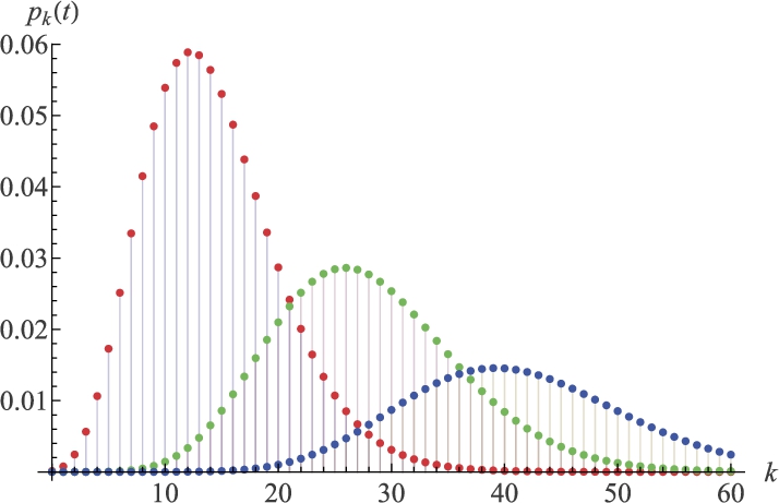
Simulation of compound Poisson processes

• Simulation of compound Poisson processes is a valuable tool for actuaries, as it allows for the generation of synthetic data that can be used to analyze the behavior of the process under various scenarios
• Simulated data can help in assessing the impact of changes in the underlying assumptions, evaluating the performance of different estimation techniques, and validating the results of analytical models
• Simulation also enables the computation of complex risk measures and the study of rare events, which may be difficult to observe in historical data

Simulation algorithms and techniques

• The basic simulation algorithm for a compound Poisson process involves generating the number of events from a Poisson distribution and then generating the severity of each event from the specified distribution
• Inverse transform sampling and acceptance-rejection methods are commonly used techniques for generating random variates from the severity distribution
• Variance reduction techniques, such as antithetic variates or control variates, can be employed to improve the efficiency and accuracy of the simulation

Monte Carlo methods

• Monte Carlo methods are a class of simulation techniques that rely on repeated random sampling to estimate the properties of a system or process
• In the context of compound Poisson processes, Monte Carlo methods can be used to estimate the distribution of aggregate losses, compute risk measures, and assess the impact of different risk management strategies
• The accuracy of Monte Carlo estimates can be improved by increasing the number of simulation runs or by using more advanced sampling techniques, such as importance sampling or stratified sampling

Applications of simulated compound Poisson processes

• Simulated compound Poisson processes find applications in various areas of actuarial work, including pricing, reserving, and risk management
• For example, simulated data can be used to test the sensitivity of pricing models to changes in the underlying assumptions, such as the Poisson rate or the parameters of the severity distribution
• In reserving, simulated data can help in estimating the distribution of future claim payments and assessing the adequacy of the reserves held by the insurer
• Simulated compound Poisson processes can also be used to evaluate the effectiveness of different risk mitigation strategies, such as reinsurance arrangements or policy deductibles

Modifications to compound Poisson processes

• While the basic compound Poisson process provides a solid foundation for modeling aggregate losses, various modifications can be made to the process to better capture the specific characteristics of the risk being modeled
• These modifications allow for greater flexibility in accommodating real-world phenomena, such as the presence of excess zeros, the dependence between claim frequency and severity, or the time-varying nature of the risk
• Incorporating these modifications into the modeling process can lead to more accurate and reliable estimates of the aggregate losses and risk measures

Zero-inflated compound Poisson processes

• Zero-inflated compound Poisson processes are designed to handle situations where there is an excess of zero claims in the data, beyond what would be expected under a standard Poisson distribution
• In a zero-inflated model, the number of claims is assumed to follow a mixture of a Poisson distribution and a degenerate distribution at zero, with a mixing probability $p$
• The probability mass function of a zero-inflated Poisson distribution is given by $P(X = k) = p\mathbb{1}_{k=0} + (1-p)\frac{e^{-\lambda}\lambda^k}{k!}$ for $k = 0, 1, 2, ...$

Marked compound Poisson processes

• Marked compound Poisson processes extend the basic compound Poisson process by associating each event with a random mark, which can represent additional information about the event, such as its type, location, or severity
• The marks are assumed to be independent and identically distributed random variables, with a distribution that may depend on the time of the event
• Marked compound Poisson processes can be used to model complex risk structures, such as multi-line insurance portfolios or spatial-temporal patterns of claims

Non-homogeneous compound Poisson processes

• Non-homogeneous compound Poisson processes allow for the Poisson rate parameter to vary over time, capturing the time-dependent nature of the risk being modeled
• The Poisson rate function $\lambda(t)$ can be specified parametrically (e.g., as a linear or exponential function of time) or estimated non-parametrically from historical data
• Non-homogeneous compound Poisson processes can be used to model seasonal patterns, trend effects, or changes in the underlying risk factors over time

Generalizations of compound Poisson processes

• Compound Poisson processes can be further generalized to accommodate more complex risk structures and dependence patterns
• These generalizations provide a rich framework for modeling a wide range of real-world phenomena, from the clustering of claims to the presence of contagion effects
• Actuaries can use these generalized models to gain a deeper understanding of the risk profile and to develop more sophisticated pricing, reserving, and risk management strategies

Compound mixed Poisson processes

• Compound mixed Poisson processes introduce an additional layer of randomness by allowing the Poisson rate parameter to be a random variable itself, following a specified mixing distribution
• The mixing distribution can be chosen to capture the heterogeneity in the risk profile, such as the presence of different risk classes or the impact of unobserved risk factors
• Common mixing distributions include the gamma, inverse Gaussian, and log-normal distributions, leading to compound negative binomial, compound Poisson-inverse Gaussian, and compound Poisson-log-normal processes, respectively

Compound Cox processes

• Compound Cox processes, also known as doubly stochastic compound Poisson processes, extend the non-homogeneous compound Poisson process by allowing the Poisson rate function to be a stochastic process itself
• The Poisson rate process can be specified using a variety of stochastic models, such as a Brownian motion, an Ornstein-Uhlenbeck process, or a jump-diffusion process
• Compound Cox processes can capture the dynamic nature of the risk and the presence of external factors influencing the claim frequency, such as economic conditions or weather events

Compound renewal processes

• Compound renewal processes generalize the compound Poisson process by replacing the Poisson process governing the claim arrivals with a more general renewal process
• In a renewal process, the inter-arrival times between claims are assumed to be independent and identically distributed random variables, with a specified distribution (e.g., Erlang, Weibull, or Pareto)
• Compound renewal processes can accommodate more flexible claim arrival patterns, such as the presence of clustering or the dependence between consecutive inter-arrival times

Compound Poisson processes in actuarial applications

• Compound Poisson processes and their generalizations find extensive applications in various areas of actuarial work, from pricing and reserving to risk management and capital allocation
• These applications rely on the ability of compound Poisson processes to capture the key characteristics of the risk being modeled, such as the frequency and severity of claims, the presence of heterogeneity, and the time-dependent nature of the risk
• Actuaries use compound Poisson processes to develop data-driven solutions to real-world problems, ensuring the financial stability and solvency of insurance companies

Pricing insurance policies

• Compound Poisson processes are used in the pricing of insurance policies to determine the appropriate premium that reflects the underlying risk
• The premium is typically set as the expected value of the aggregate losses, plus a safety loading to account for the variability in the losses and to ensure the insurer's profitability
• Actuaries use compound Poisson processes to estimate the distribution of the aggregate losses, calculate risk measures, and assess the sensitivity of the premium to changes in the underlying assumptions

Calculating risk measures and premiums

• Risk measures, such as the value-at-risk (VaR) or the expected shortfall (ES), provide a quantitative assessment of the potential losses that an insurer may face over a given time horizon and at a specified confidence level
• Compound Poisson processes can be used to estimate these risk measures by simulating the aggregate losses and calculating the relevant quantiles or conditional expectations
• Premiums can be determined using the compound Poisson process, either through the expected value principle (premium = expected losses + safety loading) or more advanced pricing principles, such as the standard deviation principle or the variance principle

Reserving and loss prediction

• Reserving is the process of setting aside funds to cover the future claims that have been incurred but not yet reported (IBNR) or have been reported but not yet fully settled (RBNS)
• Compound Poisson processes can be used to model the development of claims over time, allowing actuaries to estimate the distribution of future claim payments and to assess the adequacy of the reserves
• Loss prediction involves forecasting the future claims that an insurer may face, based on historical data and expert judgment
• Compound Poisson processes, combined with time series analysis and machine learning techniques, can be used to develop accurate and reliable loss prediction models, helping insurers to anticipate and manage their future liabilities