3.1 Simple and compound interest

Simple and compound interest form the foundation of financial mathematics. These concepts govern how money grows over time and how financial products are evaluated. Actuaries rely on them constantly to analyze investments, loans, and insurance policies.

The core distinction: simple interest calculates growth based on the original principal only, while compound interest earns interest on previously accumulated interest. This difference has massive implications for long-term financial projections, and understanding it deeply is essential for actuarial work.

Simple interest fundamentals

Simple interest is the most straightforward way to calculate the cost of borrowing or the return on an investment. Interest accrues only on the original principal, never on any interest already earned.

Principal, rate, and time

Three variables drive every simple interest calculation:

• Principal ($P$): the initial amount invested or borrowed
• Interest rate ($r$): the percentage of principal charged or earned per year, expressed as a decimal in formulas (so 5% becomes 0.05)
• Time ($t$): the duration of the investment or loan, measured in years

Simple interest formula

$I = P \times r \times t$

where $I$ is the total interest earned or charged.

For example, if $P = 1{,}000$, $r = 0.05$, and $t = 3$ years:

$I = 1{,}000 \times 0.05 \times 3 = 150$

Accumulated value calculation

The accumulated value ($A$) is the principal plus all interest earned:

$A = P + I = P(1 + rt)$

Using the same example:

$A = 1{,}000(1 + 0.05 \times 3) = 1{,}000(1.15) = 1{,}150$

Notice that the accumulated value grows linearly with time. Each year adds the same fixed amount of interest (here, $50/year).

Compound interest basics

With compound interest, interest is earned on both the principal and all previously accumulated interest. This is how most real-world financial products actually work.

Compounding frequency

Compounding frequency ($n$) is the number of times per year that interest is calculated and added to the balance. Common values:

• Annually: $n = 1$
• Semi-annually: $n = 2$
• Quarterly: $n = 4$
• Monthly: $n = 12$
• Daily: $n = 365$

Higher compounding frequency means interest gets added to the balance more often, so each subsequent compounding period applies interest to a slightly larger amount. The result: higher accumulated values.

Compound interest formula

$A = P\left(1 + \frac{r}{n}\right)^{nt}$

where $A$ is the accumulated value, $P$ is the principal, $r$ is the annual nominal rate, $n$ is the compounding frequency, and $t$ is time in years.

For example, if $P = 1{,}000$, $r = 0.05$, $n = 4$ (quarterly), and $t = 3$ years:

$A = 1{,}000\left(1 + \frac{0.05}{4}\right)^{4 \times 3} = 1{,}000(1.0125)^{12} = 1{,}161.18$

Accumulated value with compound interest

Compare that $1,161.18 to the $1,150 from simple interest on the same terms. The difference ($11.18) comes entirely from earning interest on interest. Over short periods the gap is small, but compound growth is exponential, so the gap widens dramatically over longer time horizons.

Comparing simple vs compound interest

Growth of $1 over time

Tracking how $1 grows at a given rate highlights the structural difference:

• Simple interest: $A = 1 + rt$ (linear growth, a straight line)
• Compound interest: $A = \left(1 + \frac{r}{n}\right)^{nt}$ (exponential growth, a curve that steepens over time)

At short durations the two are nearly identical. Over long durations, compound interest pulls far ahead.

Break-even point

For periods shorter than one compounding cycle, simple interest can actually produce a slightly higher accumulated value than compound interest (depending on how the partial-period calculation is handled). The break-even point is the time at which both methods yield the same accumulated value:

$1 + rt = \left(1 + \frac{r}{n}\right)^{nt}$

For an annual rate of 8% compounded quarterly, this break-even occurs at approximately $t = 1.01$ years. Beyond that point, compound interest always wins.

Advantages and disadvantages

• Simple interest is easier to calculate and transparent, but it understates the true growth of money over longer periods.
• Compound interest reflects how money actually grows in most financial products, but requires more careful calculation. Actuaries default to compound interest for nearly all real-world modeling.

Effective and nominal rates

When comparing financial products with different compounding frequencies, you need a common basis. That's where effective and nominal rates come in.

Nominal interest rate definition

The nominal interest rate ($r_{nominal}$) is the stated annual rate before accounting for compounding. A bank advertising "6% compounded monthly" is quoting a nominal rate of 6%. The actual annual return will be higher because of monthly compounding.

Effective annual rate (EAR)

The effective annual rate captures the true annual return after compounding. It answers: "If I invested $1 for exactly one year, what would my actual percentage gain be?"

$EAR = \left(1 + \frac{r_{nominal}}{n}\right)^{n} - 1$

For a nominal rate of 6% compounded monthly:

$EAR = \left(1 + \frac{0.06}{12}\right)^{12} - 1 = (1.005)^{12} - 1 = 0.06168 \approx 6.17\%$

The EAR is always greater than or equal to the nominal rate (they're equal only when $n = 1$).

Converting between nominal and effective rates

• Nominal to effective: $EAR = \left(1 + \frac{r_{nominal}}{n}\right)^{n} - 1$
• Effective to nominal: $r_{nominal} = n\left[(1 + EAR)^{\frac{1}{n}} - 1\right]$

These conversions let you compare products on equal footing. For instance, is 5.9% compounded daily better or worse than 6.0% compounded semi-annually? Convert both to EAR and compare directly.

Continuous compounding

Continuous compounding is the theoretical limit of compound interest as the compounding frequency approaches infinity. It's widely used in actuarial theory and mathematical finance.

Continuous compounding formula

$A = Pe^{rt}$

where $e \approx 2.71828$ is Euler's number.

For $P = 1{,}000$, $r = 0.05$, and $t = 3$ years:

$A = 1{,}000 \cdot e^{0.05 \times 3} = 1{,}000 \cdot e^{0.15} = 1{,}161.83$

Notice this is slightly higher than the quarterly-compounded result ($1,161.18), since continuous compounding represents the maximum possible growth for a given nominal rate.

Natural logarithm in continuous compounding

The natural logarithm ($\ln$) is the inverse of $e^x$, so you use it to solve for unknowns in continuous compounding problems.

Example: How long to double your money at 5% continuous compounding?

1. Start with $e^{rt} = 2$
2. Take $\ln$ of both sides: $rt = \ln(2)$
3. Solve for $t$: $t = \frac{\ln(2)}{r} = \frac{0.6931}{0.05} = 13.86$ years

This is closely related to the Rule of 70 approximation: doubling time $\approx \frac{70}{r\%}$.

$e$ in continuous compounding

The constant $e$ arises naturally from the limit:

$\lim_{n \to \infty} \left(1 + \frac{r}{n}\right)^{nt} = e^{rt}$

As you compound more and more frequently, the accumulated value converges to $e^{rt}$. This is why $e$ appears throughout actuarial mathematics and mathematical finance: it's the natural base for modeling continuous growth.

Applications of interest

Loans and mortgages

Interest represents the cost of borrowing. Actuaries use interest calculations to build amortization schedules that break each payment into principal and interest components, calculate monthly payments, and assess how rate changes affect borrowers over the life of a loan.

Savings accounts and CDs

Savings accounts and certificates of deposit (CDs) earn interest over time. Comparing these products requires attention to the compounding frequency and the effective annual rate, not just the advertised nominal rate.

Bonds and securities

Bonds pay interest (called coupon payments) to investors on a fixed schedule. Actuaries price bonds by discounting future cash flows back to the present, calculate yields, and assess interest rate risk on fixed-income portfolios.

Present and future value

Time value of money

A dollar today is worth more than a dollar in the future because today's dollar can be invested and earn interest. This is the time value of money, and it's the reason we discount future cash flows. Every actuarial valuation depends on this principle.

Present value formula

Present value answers: "What is a future sum worth in today's dollars?"

$PV = \frac{FV}{(1 + r)^{t}}$

For example, the present value of $1,000 to be received in 5 years at a 6% annual discount rate:

$PV = \frac{1{,}000}{(1.06)^{5}} = \frac{1{,}000}{1.33823} = 747.26$

This means you'd need to invest $747.26 today at 6% to have $1,000 in five years.

Future value formula

Future value answers: "What will today's money be worth later?"

$FV = PV(1 + r)^{t}$

Plugging in $PV = 747.26$, $r = 0.06$, $t = 5$:

$FV = 747.26(1.06)^{5} = 1{,}000$

Present and future value are simply inverses of each other.

Annuities and perpetuities

Annuities and perpetuities are series of recurring payments. They show up constantly in actuarial work: pension benefits, insurance premiums, loan repayments, and structured settlements.

Ordinary annuity vs annuity due

• Ordinary annuity: payments occur at the end of each period (most loans work this way)
• Annuity due: payments occur at the beginning of each period (rent payments, insurance premiums)

The timing difference matters because annuity-due payments each have one extra period to earn interest, making an annuity due more valuable than an otherwise identical ordinary annuity.

Present value of an annuity

Ordinary annuity:

$PV = PMT \times \frac{1 - (1 + r)^{-n}}{r}$

Annuity due:

$PV = PMT \times \frac{1 - (1 + r)^{-n}}{r} \times (1 + r)$

where $PMT$ is the periodic payment, $r$ is the interest rate per period, and $n$ is the total number of payments.

The annuity-due formula is just the ordinary annuity formula multiplied by $(1 + r)$, reflecting that each payment is received one period earlier.

Perpetuity formula and examples

A perpetuity is an annuity that continues forever. Its present value simplifies to:

$PV = \frac{PMT}{r}$

For a perpetuity paying $1,000 annually at a 5% discount rate:

$PV = \frac{1{,}000}{0.05} = 20{,}000$

This means a lump sum of $20,000 invested at 5% could fund $1,000 annual payments indefinitely. Perpetuities appear in endowment valuations, preferred stock pricing, and certain actuarial reserve calculations.

Solving interest-related problems

Determining time, rate, or principal

Most exam problems give you all but one variable and ask you to solve for it. The approach is always the same: pick the right formula, plug in what you know, and isolate the unknown.

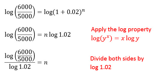
Example: How long to double an investment at 8% compounded annually?

1. Set up: $2P = P(1 + 0.08)^{t}$
2. Divide both sides by $P$: $2 = (1.08)^{t}$
3. Take $\ln$ of both sides: $\ln(2) = t \cdot \ln(1.08)$
4. Solve: $t = \frac{\ln(2)}{\ln(1.08)} = \frac{0.6931}{0.07696} = 9.006$ years

Interest rate comparison and analysis

To compare products with different compounding frequencies, convert everything to the effective annual rate (EAR). The product with the higher EAR delivers the better return, regardless of how the nominal rate is quoted.

Calculating periodic payments

To find the payment needed to pay off a loan or reach a savings goal, rearrange the annuity formula to solve for $PMT$.

Example: Monthly payment on a $100,000 loan at 6% annual interest over 5 years.

1. Convert to monthly terms: $r = \frac{0.06}{12} = 0.005$, $n = 5 \times 12 = 60$
2. Use the present value of an ordinary annuity formula, solving for $PMT$:

$PMT = PV \times \frac{r}{1 - (1 + r)^{-n}} = 100{,}000 \times \frac{0.005}{1 - (1.005)^{-60}}$

1. Calculate: $(1.005)^{-60} = 0.74137$, so the denominator is $1 - 0.74137 = 0.25863$

2. Result: $PMT = 100{,}000 \times \frac{0.005}{0.25863} = 1{,}933.28$

The monthly payment is approximately $1,933.28.