Time series analysis gives actuaries a framework for predicting future trends in insurance claims, premiums, and reserves. By examining data collected over time, you can identify patterns and relationships that drive informed decisions and effective risk management.
This topic covers the key components of time series data (trend, seasonal, cyclical, and irregular), the concept of stationarity, autocorrelation tools, and the major model families: AR, MA, ARMA, ARIMA, and SARIMA.
Components of time series
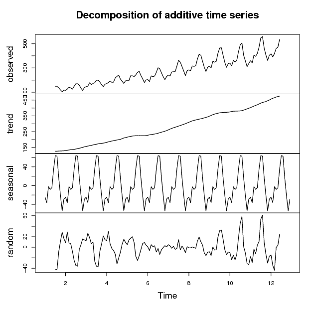
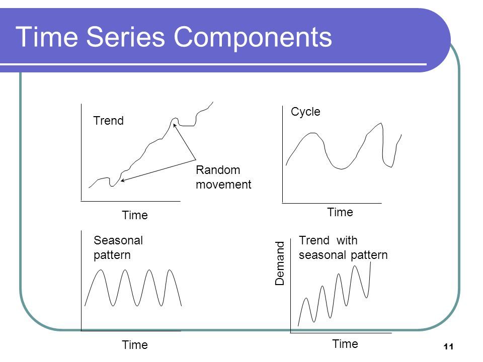
A time series is simply a sequence of observations recorded at regular intervals: daily stock prices, monthly sales figures, annual insurance claims. Time series analysis examines these observations to uncover patterns that are useful for actuarial forecasting. Each time series can be decomposed into four components.
Trend component
- The long-term increase or decrease in the data over time.
- Can be linear (constant rate of change) or non-linear (varying rate of change).
- Examples:
- Increasing average life expectancy affecting life insurance pricing
- A decreasing trend in automotive theft reducing auto insurance claims over decades
Seasonal component
- Predictable fluctuations tied to calendar-based factors (day of week, month, quarter).
- These patterns repeat at fixed intervals. Think of insurance claims rising in winter months due to weather-related accidents, or retail sales peaking during holiday seasons.
- Identifying seasonal components helps actuaries adjust forecasts and pricing strategies accordingly.
Cyclical component
- Medium to long-term fluctuations around the trend, typically lasting 2+ years.
- Unlike seasonal patterns, cycles are not fixed in length or magnitude.
- Often tied to economic or business cycles:
- Economic downturns leading to increased unemployment insurance claims
- Market cycles affecting investment returns and pension fund valuations
Irregular component
- Unpredictable, random fluctuations not captured by the other three components.
- Caused by one-off events or measurement errors:
- Natural disasters causing spikes in property insurance claims
- Data entry errors or reporting delays creating anomalies in claims data
Stationarity in time series
Many time series models assume that the statistical properties of the data remain constant over time. This property is called stationarity, and assessing it is one of the first steps before fitting a model. If your data isn't stationary, you'll need to transform it before modeling.
Strict vs weak stationarity
- Strict stationarity: the entire joint probability distribution of the time series is invariant under time shifts. This is rarely assumed in practice because it's extremely difficult to verify.
- Weak stationarity (covariance stationarity): only requires that the mean, variance, and autocovariance remain constant over time. This is the version you'll work with most often. It demands that the first two moments (mean and variance) be time-invariant.
Testing for stationarity
- Visual inspection of time series plots can give you initial clues (look for obvious trends or changing variance).
- Formal statistical tests include:
- Augmented Dickey-Fuller (ADF) test: tests the null hypothesis that a unit root is present (non-stationary)
- KPSS test: tests the null hypothesis that the series is stationary (note the reversed null compared to ADF)
- Phillips-Perron (PP) test: similar to ADF but more robust to serial correlation in the error terms
- Using ADF and KPSS together is a common strategy since their opposing null hypotheses give you a more complete picture.
Transforming non-stationary series
- Differencing: computing differences between consecutive observations to remove trend and stabilize the mean.
- First-order differencing:
- Higher-order differencing may be needed for more complex trends.
- Log transformations: applying logarithms to stabilize the variance when it grows proportionally with the level of the series.
- Seasonal differencing: removing seasonal components by computing differences between observations separated by the seasonal period (e.g., for monthly data with annual seasonality).
Autocorrelation and partial autocorrelation
These two functions are your primary diagnostic tools for identifying which type of model to fit. Autocorrelation measures the linear relationship between a time series and its own lagged values. Partial autocorrelation measures that same relationship but controls for the effects of all intermediate lags.
Autocorrelation function (ACF)
- The ACF plots autocorrelation coefficients against the lag order.
- Autocorrelation at lag :
- For a weakly stationary series, this simplifies to , where is the autocovariance at lag .
- Significant spikes in the ACF plot indicate meaningful autocorrelation at those lags.
Partial autocorrelation function (PACF)
- The PACF plots partial autocorrelation coefficients against the lag order.
- The partial autocorrelation at lag is the correlation between and after removing the linear effects of .
- This is especially useful for identifying the order of autoregressive terms.
Interpreting ACF and PACF plots
The decay patterns in these plots tell you which model family to consider:
| Pattern | ACF | PACF | Suggested Model |
|---|---|---|---|
| AR(p) | Decays gradually (exponential or oscillating) | Cuts off after lag | Autoregressive |
| MA(q) | Cuts off after lag | Decays gradually | Moving average |
| ARMA(p, q) | Both decay gradually | Both decay gradually | Mixed model |
"Cuts off" means the values drop to statistically insignificant levels abruptly. "Decays gradually" means they taper toward zero over many lags.
Autoregressive (AR) models
AR models express the current value of a time series as a linear combination of its own past values plus a white noise error term. They're well-suited for series where the current observation clearly depends on recent history.
AR(p) model structure
- : current value of the time series
- : constant term
- : autoregressive coefficients
- : white noise error term (mean zero, constant variance)
- The order determines how many lagged terms are included.
For stationarity, the roots of the characteristic polynomial must all lie outside the unit circle.
Estimating AR model parameters
- Ordinary least squares (OLS): treats lagged values as regressors; straightforward but assumes no serial correlation in errors.
- Maximum likelihood estimation (MLE): more efficient, especially for smaller samples.
- Yule-Walker equations: exploit the relationship between autocovariances and AR coefficients; computationally convenient.
Selecting AR model order
- PACF: the lag at which the PACF cuts off suggests the appropriate order .
- Information criteria: AIC or BIC. Lower values indicate a better trade-off between model fit and complexity. BIC tends to favor more parsimonious models than AIC because it penalizes additional parameters more heavily.
Moving average (MA) models
MA models express the current value as a linear combination of the current and past white noise error terms. They capture short-term dependencies where shocks to the system persist for a limited number of periods.
MA(q) model structure
- : current value of the time series
- : mean of the time series
- : moving average coefficients
- : white noise error terms
- The order determines how many lagged error terms are included.
MA models are always weakly stationary regardless of the coefficient values. For invertibility (which ensures unique parameter estimates), the roots of must lie outside the unit circle.
Estimating MA model parameters
- Maximum likelihood estimation (MLE): the most common approach.
- Conditional least squares (CLS): conditions on initial error values.
- Method of moments (MM): matches sample autocovariances to theoretical ones.
Estimation is more complex than for AR models because the error terms are not directly observed.
Selecting MA model order
- ACF: the lag at which the ACF cuts off suggests the appropriate order .
- Information criteria: AIC or BIC, with lower values preferred.
Autoregressive moving average (ARMA) models
ARMA models combine AR and MA components to capture both the autoregressive structure and the moving average behavior in a single stationary model. They're more flexible than either AR or MA alone.
ARMA(p, q) model structure
- : constant term
- : autoregressive coefficients
- : moving average coefficients
- : white noise error term
- The orders and determine the number of AR and MA terms.
ARMA models require the series to be stationary. If it isn't, you need to difference first (which leads to ARIMA).
Estimating ARMA model parameters
- Maximum likelihood estimation (MLE): most widely used.
- Conditional least squares (CLS): computationally simpler but less efficient.
- Hannan-Rissanen algorithm: a two-stage method that first fits a high-order AR to estimate residuals, then uses those residuals to estimate the ARMA parameters.
Estimation is more involved than for pure AR or MA models because the AR and MA components interact.
Selecting ARMA model order
- ACF and PACF plots: when both decay gradually rather than cutting off, an ARMA model is indicated. The specific rates of decay can suggest starting values for and .
- Information criteria: fit several candidate ARMA(p, q) models and choose the one with the lowest AIC or BIC.
- In practice, you often try a grid of small and values (e.g., 0 to 3 each) and compare.
Autoregressive integrated moving average (ARIMA) models
ARIMA models extend ARMA to handle non-stationary time series by incorporating a differencing step. The "I" stands for "integrated," referring to the fact that the stationary ARMA process must be summed (integrated) back to recover the original series.
ARIMA(p, d, q) model structure
- : order of the autoregressive component
- : degree of differencing needed to achieve stationarity
- : order of the moving average component
- : the backshift operator, where
- : autoregressive coefficients
- : moving average coefficients
- : constant term
- : white noise error term
Note that when , the ARIMA model reduces to a standard ARMA model.
Differencing for non-stationarity
Differencing removes trend from a non-stationary series. The degree tells you how many rounds of differencing are needed:
-
First-order differencing: (removes a linear trend)
-
Second-order differencing: (removes a quadratic trend)
-
After differencing, check for stationarity again using ADF/KPSS tests.
-
Once stationary, model the differenced series as an ARMA(p, q) process.
In practice, or is almost always sufficient. If you need , reconsider whether the data needs a different transformation.
Estimating ARIMA model parameters
- Maximum likelihood estimation (MLE): standard approach.
- Conditional least squares (CLS): conditions on initial values.
- Box-Jenkins methodology: an iterative three-stage process:
- Identification: use ACF/PACF of the differenced series to propose candidate and values.
- Estimation: fit the model and estimate parameters.
- Diagnostic checking: examine residuals to verify they resemble white noise.
Selecting ARIMA model order
- Determine first by differencing until the series passes stationarity tests.
- Then use ACF and PACF plots of the differenced series to identify and .
- Compare candidate models using AIC or BIC (lower is better).
- Iterate: if diagnostics reveal problems, revise the model orders and re-estimate.
Seasonal ARIMA (SARIMA) models
SARIMA models extend ARIMA to capture both non-seasonal and seasonal patterns. They're the go-to model for actuarial data with clear seasonal structure, such as monthly claims data or quarterly premium volumes.
SARIMA(p, d, q)(P, D, Q)m model structure
- : orders of the non-seasonal AR, differencing, and MA components
- : orders of the seasonal AR, differencing, and MA components
- : number of periods per season (e.g., for monthly data with annual seasonality)
- : non-seasonal AR and MA polynomials in
- : seasonal AR and MA polynomials in
- : constant term
- : white noise error term
The notation looks dense, but the idea is straightforward: you're fitting an ARIMA model for the non-seasonal behavior and a separate ARIMA-like model for the seasonal behavior, then multiplying them together.
Seasonal differencing
- Seasonal differencing removes the seasonal component:
- First-order seasonal differencing:
- For monthly data with annual seasonality, this means subtracting the value from 12 months ago.
- You may need both regular differencing (to remove trend) and seasonal differencing (to remove seasonality).
Estimating SARIMA model parameters
- MLE and CLS remain the standard estimation methods.
- The Box-Jenkins methodology applies here too, with the added step of examining seasonal lags in the ACF and PACF.
- Estimation is iterative: identify, estimate, diagnose, and refine.
Selecting SARIMA model order
- Apply seasonal differencing () and regular differencing () until the series is stationary.
- Examine the ACF and PACF at non-seasonal lags (1, 2, 3, ...) to determine and .
- Examine the ACF and PACF at seasonal lags () to determine and .
- Fit candidate models and compare using AIC or BIC.
- Check residual diagnostics and refine as needed.
Model diagnostics and validation
After fitting a model, you need to verify that it adequately captures the dynamics of the data and will produce reliable forecasts. Diagnostics focus on the residuals: if the model is well-specified, the residuals should behave like white noise.
Residual checks:
- Plot the residuals over time and look for remaining patterns or non-constant variance.
- Examine the ACF of the residuals. Significant spikes indicate the model hasn't captured all the autocorrelation structure.
- Ljung-Box test: a formal test for whether a group of autocorrelations in the residuals are jointly zero. A significant p-value suggests the model is inadequate.
Model comparison:
- Use AIC and BIC to compare competing models on the same dataset. These criteria balance goodness of fit against model complexity.
- Out-of-sample validation: hold back a portion of the data (e.g., the last 12 months), fit the model on the remaining data, and compare forecasts to actual values. Common accuracy metrics include Mean Absolute Error (MAE), Root Mean Squared Error (RMSE), and Mean Absolute Percentage Error (MAPE).
Common pitfalls to watch for:
- Overfitting: a model with too many parameters may fit the training data well but forecast poorly. Prefer simpler models when AIC/BIC values are close.
- Under-differencing: residuals that still show a trend or seasonal pattern indicate you haven't differenced enough.
- Over-differencing: can introduce unnecessary complexity and artificial patterns in the residuals.