Fundamentals of Mean Field Theory
Mean field theory tackles a core problem in statistical mechanics: how do you analyze a system where every particle interacts with every other particle? The answer is to replace all those complicated pairwise interactions with a single average "effective field" that each particle feels. This converts an intractable many-body problem into a solvable single-body problem.
The trade-off is that you lose information about local correlations and fluctuations. But for many systems, especially those with long-range interactions or high coordination numbers, mean field theory captures the essential physics of phase transitions and collective behavior remarkably well.
Definition and Basic Concepts
The central idea: instead of tracking how spin interacts with each of its neighbors individually, you assume every spin sees the same average environment produced by all the others.
- Each particle interacts with an effective field rather than with individual neighbors
- The many-body problem reduces to a self-consistent single-particle problem
- Fluctuations and correlations between particles are neglected by construction
- Despite this simplification, the theory often gives qualitatively correct predictions for phase transitions and symmetry breaking
Assumptions and Limitations
Mean field theory rests on the assumption that the local environment of each particle is well-represented by the global average. This works when:
- Interactions are long-range, so each particle couples to many others and local deviations average out
- The spatial dimension is high, giving each site many neighbors (the theory becomes exact as )
- The system is far from a critical point, where fluctuations are small
It breaks down when:
- Short-range correlations dominate the physics (low-dimensional systems)
- The system is near a critical point, where fluctuations diverge and the correlation length grows large
- You need accurate critical exponents, which mean field theory systematically gets wrong below the upper critical dimension
Mean Field Approximation Techniques
Several methods exist for implementing the mean field approximation. Each offers a different balance of accuracy, computational cost, and physical transparency.
Variational Approach
This method uses the Bogoliubov inequality to bound the true free energy from above. You choose a trial Hamiltonian (usually non-interacting) with adjustable parameters, then minimize the resulting free energy.
-
Write a trial Hamiltonian with variational parameters (e.g., an effective field )
-
Compute the variational free energy: , where denotes the average over the trial ensemble
-
Minimize with respect to the variational parameters
-
The result provides an upper bound on the true free energy
This is the basis of the Hartree-Fock approximation in quantum many-body theory. Adding more variational parameters (e.g., Jastrow factors for correlations) systematically improves accuracy.
Effective Field Method
This is the most physically intuitive approach, often introduced through Weiss molecular field theory for magnets.
- Pick a single spin in the lattice
- Replace all neighboring spins with their thermal average: (the magnetization)
- The spin now sits in an effective field , where is the coordination number, is the coupling constant, and is any external field
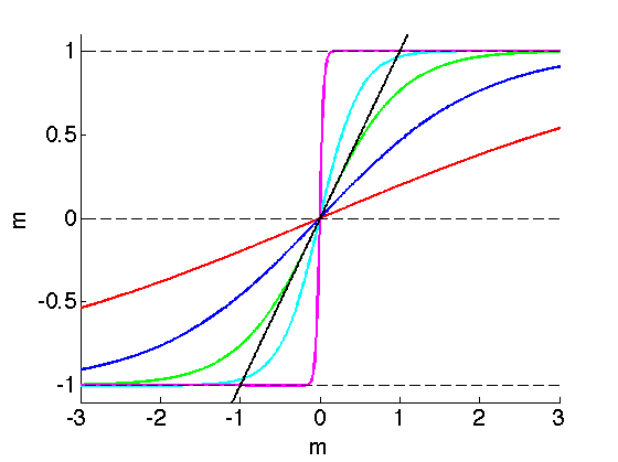
- Compute for the Ising model, giving a self-consistency equation
- Solve this equation (graphically or numerically) to find the equilibrium magnetization
The self-consistency requirement is what makes this a mean field theory: the average field depends on , and depends on the average field.
Cluster Expansion
Rather than treating each site independently, cluster methods group nearby sites together and treat intra-cluster interactions exactly while applying the mean field approximation only to inter-cluster couplings.
- Systematically includes short-range correlations that simple mean field theory misses
- The Bethe-Peierls approximation (Bethe lattice) is the simplest cluster method, treating a central spin and its neighbors exactly
- Higher-order cluster methods (Cluster Variation Method, or CVM) include larger groups of sites
- Truncating at different cluster sizes gives a hierarchy of increasingly accurate approximations
- Widely used in alloy thermodynamics and lattice gas models
Applications in Statistical Mechanics
Ising Model
The Ising model, with spins on a lattice interacting via , is the standard testbed for mean field theory.
- Mean field predicts a second-order phase transition at , where is the coordination number
- In 1D (), mean field incorrectly predicts a transition; the exact result shows no phase transition at finite temperature
- In 2D, the exact Onsager solution gives for a square lattice (), while mean field predicts , overshooting by about 76%
- Mean field becomes increasingly accurate as increases, and is exact for
This model cleanly illustrates both the qualitative successes and quantitative failures of the approximation.
Ferromagnetic Systems
Below the Curie temperature , mean field theory predicts spontaneous magnetization even without an external field. The magnetization near follows:
This square-root behavior (exponent ) is a signature of mean field theory. Real 3D ferromagnets have , showing that fluctuations matter near the critical point.
- The predicted scales with the coordination number , which is qualitatively correct: more neighbors means stronger collective ordering
- The overall shape of the magnetization curve is qualitatively right
- The theory extends naturally to antiferromagnets (using sublattice magnetizations) and more complex magnetic orderings
Liquid-Gas Transitions
The van der Waals equation is a classic mean field theory for fluids:
Here accounts for the average attractive interaction between molecules, and for their finite volume. This equation predicts a critical point and a liquid-gas coexistence curve, capturing the qualitative phase diagram of real fluids. However, it gives the same mean field critical exponents (, ) that fail quantitatively near the critical point.
Mathematical Formulation
Mean Field Equations
The self-consistency equation is the heart of any mean field theory. For the Ising model with coordination number and coupling :
where is the magnetization per spin and is the external field.
- At , this equation has a non-trivial solution () only below
- Near , you can expand the to find the scaling of with temperature
- These transcendental equations are typically solved graphically (plotting both sides vs. ) or numerically
- More complex systems yield coupled self-consistency equations for multiple order parameters
Free Energy Calculations
The mean field free energy for the Ising model can be written as a function of :
Near the critical point, this can be expanded in powers of to obtain the Landau form:
The sign change of the quadratic coefficient at signals the phase transition. Minimizing with respect to recovers the self-consistency equation and determines the equilibrium state.
Order Parameters
An order parameter is a quantity that distinguishes the ordered phase from the disordered one. It's zero in the disordered (high-symmetry) phase and nonzero in the ordered (broken-symmetry) phase.
- Magnetization for ferromagnets
- Density difference for the liquid-gas transition
- Superconducting gap for superconductors
For continuous (second-order) transitions, the order parameter grows continuously from zero at . For first-order transitions, it jumps discontinuously. Near the critical point, order parameters obey scaling laws: .
Critical Phenomena and Phase Transitions
Mean Field Critical Exponents
Mean field theory predicts a set of universal critical exponents that are independent of microscopic details:
| Exponent | Definition | Mean Field Value |
|---|---|---|
| Order parameter: | 1/2 | |
| Susceptibility: $$\chi \sim | T - T_c | |
| Critical isotherm: at | 3 | |
| Specific heat: $$C \sim | T - T_c |
These values are exact above the upper critical dimension for short-range Ising-like systems. Below , fluctuations modify the exponents. For example, the 3D Ising model has , .
Universality Classes
In reality, critical exponents depend on just a few features: spatial dimensionality, symmetry of the order parameter, and range of interactions. Systems sharing these features belong to the same universality class and have identical critical exponents.
Mean field theory misses this richness entirely. It predicts a single set of exponents for all continuous transitions, regardless of dimension or symmetry. This is one of its most significant failures and a key motivation for the renormalization group.
Landau Theory Connection
Landau theory is a phenomenological approach that expands the free energy in powers of the order parameter, guided by symmetry:
- The coefficients are determined by symmetry (e.g., if the system has symmetry, only even powers appear)
- Minimizing reproduces the same critical exponents as microscopic mean field theories
- Landau theory is equivalent to mean field theory near , but it's formulated without reference to any specific microscopic model
- Adding gradient terms gives Ginzburg-Landau theory, which can describe spatial variations of the order parameter and the effects of fluctuations
Beyond Mean Field Theory
Fluctuations and Correlations
Mean field theory assumes the order parameter is spatially uniform. Near a critical point, this assumption fails badly because fluctuations grow and become correlated over long distances.
The Ginzburg criterion quantifies when mean field theory breaks down. It compares the magnitude of fluctuations to the mean field order parameter. For a -dimensional system with short-range interactions, mean field theory fails when:
where is the Ginzburg number. For 3D systems, this number can be small (mean field works over most of the phase diagram) or large (fluctuations dominate), depending on the system.
In mean field theory, correlation functions decay exponentially: . At the critical point, the true behavior is a power law: , which mean field theory cannot capture.
Renormalization Group Approach
The renormalization group (RG) is the systematic framework for handling fluctuations at all length scales. It explains why universality exists and predicts the correct critical exponents.
The basic idea: coarse-grain the system by integrating out short-wavelength fluctuations, then rescale. Fixed points of this transformation correspond to critical points, and the behavior near fixed points determines the critical exponents.
- RG reduces to mean field theory above , confirming that mean field exponents are exact there
- Below , RG predicts non-classical exponents that match experiments
- The -expansion () provides a perturbative way to compute corrections to mean field exponents
Corrections to Mean Field
Several systematic methods improve on mean field predictions:
- High-temperature and low-temperature series expansions: compute thermodynamic quantities as power series in or , then extrapolate
- -expansion: expand critical exponents in powers of , where is the upper critical dimension
- Bethe-Peierls approximation: treat a cluster of spins exactly, embedding it in a mean field environment
- Effective field theories: incorporate local fluctuations while keeping the mean field structure at large scales

Numerical Methods
Monte Carlo Simulations
Monte Carlo methods sample configurations stochastically, weighted by the Boltzmann factor, to compute thermal averages without solving the partition function analytically.
- Start from an initial configuration
- Propose a move (e.g., flip a spin)
- Accept or reject the move based on the Metropolis criterion: accept if ; if , accept with probability
- Repeat to generate a Markov chain of configurations
- Compute averages over the chain after equilibration
Monte Carlo provides numerically exact results (within statistical error) for finite systems and serves as a benchmark for testing mean field predictions. It can handle complex geometries and interactions that are analytically intractable.
Molecular Dynamics vs. Mean Field
Molecular dynamics (MD) integrates Newton's equations for all particles, giving access to both equilibrium and dynamical properties. Compared to mean field theory:
- MD captures the full microscopic dynamics, including correlations and fluctuations
- It's far more computationally expensive, scaling with system size and simulation time
- MD can validate or refute mean field predictions for specific systems
- Hybrid approaches like Car-Parrinello molecular dynamics combine quantum mean field (density functional theory) with classical dynamics for the nuclei
Strengths and Weaknesses
Accuracy vs. Simplicity
Mean field theory's greatest strength is that it provides a qualitatively correct picture of phase transitions with minimal computational effort. You get the existence of a critical temperature, spontaneous symmetry breaking, and the general shape of the phase diagram, all from a self-consistency equation you can solve on paper.
The cost is quantitative accuracy near critical points and in low dimensions. For building intuition and guiding more detailed calculations, mean field theory remains indispensable.
Range of Validity
The Ginzburg criterion is the practical tool for assessing when mean field theory applies. As a rule of thumb:
- High dimensions ( for Ising-like systems): mean field is exact
- 3D systems far from : mean field is usually a good approximation
- 3D systems near : mean field fails for critical exponents but may still give reasonable transition temperatures
- 2D and 1D systems: mean field is often qualitatively wrong (e.g., predicting transitions that don't exist in 1D)
- Long-range interactions: extend the range of validity, effectively increasing the "effective dimension"
Comparison with Exact Solutions
Where exact solutions exist, they provide a clear picture of mean field theory's accuracy:
- 1D Ising model: exact solution shows no phase transition; mean field incorrectly predicts one
- 2D Ising model (Onsager): exact and critical exponents differ significantly from mean field values
- Infinite-dimensional models: mean field becomes exact, confirming the theory's internal consistency
- Spherical model: solvable in all dimensions, with mean field exponents above
Advanced Topics
Spin Glasses and Disorder
The Sherrington-Kirkpatrick (SK) model applies mean field theory to disordered magnetic systems where couplings are random. The physics is dramatically richer than the ferromagnetic case:
- The free energy landscape has an exponential number of metastable states
- Replica symmetry breaking (Parisi's solution) is needed to correctly describe the low-temperature phase
- The mathematical structure connects to optimization problems, computational complexity, and neural network theory
- This is one of the rare cases where mean field theory reveals genuinely new physics rather than just approximating known behavior
Quantum Mean Field Theory
Mean field ideas extend naturally to quantum systems:
- Hartree-Fock: replaces electron-electron interactions with an average potential; each electron moves in the self-consistent field of all others
- Bogoliubov theory: treats weakly interacting Bose gases by replacing the condensate with a classical field
- Density functional theory (DFT): maps the interacting electron problem to a non-interacting one in an effective potential (Kohn-Sham scheme)
- Dynamical mean field theory (DMFT): maps a lattice problem to a self-consistent impurity problem, capturing local quantum fluctuations while treating spatial correlations at the mean field level. This is particularly powerful for strongly correlated electron systems.
Non-Equilibrium Systems
Mean field approximations also apply outside equilibrium:
- Reaction-diffusion systems: replace spatial correlations with average concentrations to get rate equations
- Boltzmann equation: a mean field kinetic theory where the collision term depends on the single-particle distribution function
- Fokker-Planck equations: describe the evolution of probability distributions under stochastic dynamics
- Applications range from polymer dynamics to epidemiology (e.g., SIR models where infection rates depend on average population fractions)