10.2 Kullback-Leibler divergence

Definition of Kullback-Leibler divergence

Kullback-Leibler divergence (KL divergence) measures how one probability distribution differs from a second, reference distribution. In statistical mechanics, this matters because you're constantly approximating complex true distributions with simpler models, and KL divergence tells you exactly how much information you lose in that approximation.

Think of it this way: if $P$ is the true distribution of microstates in your system and $Q$ is your model's approximation, KL divergence quantifies the price you pay for using $Q$ instead of $P$.

Mathematical formulation

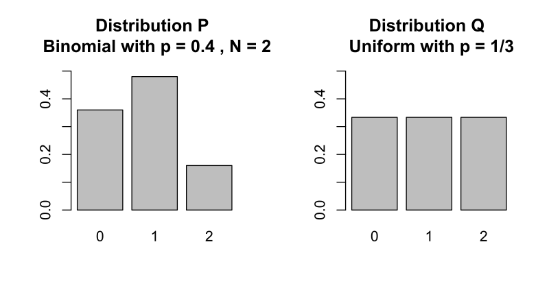
For discrete probability distributions:

$D_{KL}(P \| Q) = \sum_{i} P(i) \log \frac{P(i)}{Q(i)}$

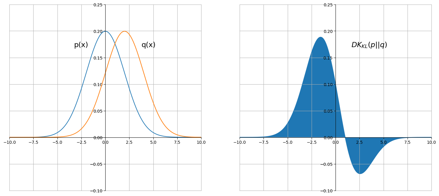
For continuous distributions:

$D_{KL}(P \| Q) = \int_{-\infty}^{\infty} p(x) \log \frac{p(x)}{q(x)} \, dx$

Two critical properties follow directly from the definition:

• Non-negativity: $D_{KL}(P \| Q) \geq 0$ always, a consequence of Jensen's inequality applied to the concavity of the logarithm.
• Zero condition: $D_{KL}(P \| Q) = 0$ if and only if $P$ and $Q$ are identical distributions (almost everywhere).

The logarithm base determines the units: base 2 gives bits, base $e$ gives nats. In statistical mechanics, natural logarithms (nats) are standard.

Interpretation as relative entropy

KL divergence is often called relative entropy, and the name reveals its meaning. It measures the extra information needed to encode samples from $P$ using a code optimized for $Q$.

Suppose you design an optimal coding scheme assuming distribution $Q$. If the data actually follows $P$, you'll need extra bits on average to encode each sample. That average excess cost is exactly $D_{KL}(P \| Q)$.

Another useful way to think about it: KL divergence captures the average "surprise" you experience when observing data drawn from $P$ while expecting $Q$. The greater the mismatch between the two distributions, the more surprised you are, and the larger the divergence.

Properties of KL divergence

• Asymmetry: $D_{KL}(P \| Q) \neq D_{KL}(Q \| P)$ in general. This means KL divergence is not a true distance metric. The order of arguments matters, and you need to be deliberate about which distribution is $P$ and which is $Q$.
• No triangle inequality: Another reason it fails to be a metric.
• Additivity for independent distributions: If $P_1, P_2$ are independent and $Q_1, Q_2$ are independent, then $D_{KL}(P_1 P_2 \| Q_1 Q_2) = D_{KL}(P_1 \| Q_1) + D_{KL}(P_2 \| Q_2)$. This mirrors how entropy is additive for independent subsystems.
• Invariance under reparametrization: KL divergence doesn't change if you apply an invertible transformation to the random variable.

Applications in statistical mechanics

Free energy calculations

KL divergence connects directly to free energy. If $P$ is the true equilibrium (Boltzmann) distribution and $Q$ is a trial distribution, you can show that:

$F_Q - F = k_B T \, D_{KL}(Q \| P)$

where $F$ is the true free energy and $F_Q$ is the variational free energy associated with $Q$. Because KL divergence is non-negative, this gives you the Bogoliubov inequality: $F_Q \geq F$. Minimizing $D_{KL}(Q \| P)$ over a family of trial distributions is the basis of variational free energy methods.

KL divergence also appears in the Jarzynski equality, where it helps quantify the dissipated work in irreversible processes. The average dissipation during a non-equilibrium process relates to the KL divergence between the forward and reverse path distributions.

Model comparison

When you have competing statistical mechanical models for a system, KL divergence quantifies how well each model's predicted distribution matches the observed data. A model with smaller KL divergence from the empirical distribution captures more of the system's statistical structure.

This connects to Bayesian model selection: the evidence ratio between two models relates to their relative KL divergences from the true distribution. The principle at work is a formal version of Occam's razor, where you penalize unnecessary model complexity.

Information theory connections

KL divergence sits at the intersection of statistical mechanics and information theory:

• Thermodynamic entropy and Shannon entropy: For a system at equilibrium, the Gibbs entropy $S = -k_B \sum_i p_i \ln p_i$ has the same functional form as Shannon entropy (up to the Boltzmann constant). KL divergence from the uniform distribution recovers the difference between maximum entropy and actual entropy.
• Maxwell's demon: The demon's ability to reduce entropy requires acquiring information about molecular states. KL divergence quantifies the information gained, and Landauer's principle states that erasing this information dissipates at least $k_B T \ln 2$ of heat per bit. The demon can't beat the second law.
• Fundamental limits: The minimum thermodynamic cost of any computation or measurement is bounded by information-theoretic quantities expressible through KL divergence.

Relationship to other concepts

KL divergence vs. cross-entropy

Cross-entropy between $P$ and $Q$ is defined as:

$H(P, Q) = -\sum_{i} P(i) \log Q(i)$

The relationship to KL divergence is clean:

$D_{KL}(P \| Q) = H(P, Q) - H(P)$

Since $H(P)$ (the entropy of the true distribution) is a constant with respect to $Q$, minimizing cross-entropy and minimizing KL divergence over $Q$ are equivalent optimization problems. This is why cross-entropy loss works as a training objective in machine learning: it's implicitly minimizing KL divergence from the data distribution.

KL divergence vs. mutual information

Mutual information between two random variables $X$ and $Y$ is itself a KL divergence:

$I(X; Y) = D_{KL}(P(X, Y) \| P(X) P(Y))$

It measures how far the joint distribution $P(X, Y)$ is from the product of marginals. If $X$ and $Y$ are independent, the joint equals the product of marginals, so $I(X; Y) = 0$. Any statistical dependence between the variables makes the mutual information positive.

In statistical mechanics, mutual information quantifies correlations between subsystems and appears in analyses of coarse-graining, where you want to know how much information about microscopic details survives in a macroscopic description.

Jensen-Shannon divergence

Because KL divergence is asymmetric, the Jensen-Shannon divergence (JSD) provides a symmetrized alternative:

$JSD(P \| Q) = \frac{1}{2} D_{KL}(P \| M) + \frac{1}{2} D_{KL}(Q \| M)$

where $M = \frac{1}{2}(P + Q)$ is the mixture distribution. JSD is bounded between 0 and $\log 2$ (or 0 and 1 when using base-2 logarithms), and its square root is a true metric. This makes it useful when you need a symmetric, bounded measure of distributional difference.

Limitations and considerations

Asymmetry of KL divergence

The asymmetry has real consequences for how you set up problems. $D_{KL}(P \| Q)$ (the "forward" KL) penalizes $Q$ heavily wherever $P$ has support but $Q$ assigns low probability. This tends to produce approximations that are mean-seeking (spreading out to cover all modes of $P$). The "reverse" KL, $D_{KL}(Q \| P)$, instead penalizes $Q$ for placing mass where $P$ doesn't, producing mode-seeking approximations that lock onto a single peak. Choosing the wrong direction can give misleading results.

Infinite divergence cases

If $Q(i) = 0$ for any state $i$ where $P(i) > 0$, the KL divergence is infinite. Physically, this means your model $Q$ assigns zero probability to a state that actually occurs, which is infinitely "surprising." In practice, this requires:

• Ensuring the support of $Q$ covers the support of $P$
• Using smoothing techniques (e.g., adding a small $\epsilon$ to all probabilities)
• Switching to alternative divergences like JSD that handle this gracefully

Numerical stability issues

Computing KL divergence involves logarithms of potentially very small probabilities, which can cause underflow or overflow. Common remedies include:

• Working in log-space throughout the calculation
• Using the log-sum-exp trick to avoid exponentiating large numbers
• Being especially careful with high-dimensional or sparse distributions where many probabilities are near zero

Calculation methods

Discrete probability distributions

Direct computation follows the definition:

1. For each state $i$, compute $P(i) \log \frac{P(i)}{Q(i)}$
2. Handle edge cases: if $P(i) = 0$, that term contributes 0 (by convention, since $\lim_{x \to 0} x \log x = 0$). If $Q(i) = 0$ but $P(i) > 0$, the divergence is infinite.
3. Sum over all states.

This is straightforward for small state spaces and can be vectorized efficiently.

Continuous probability distributions

For continuous distributions, you have several options depending on the situation:

• Analytical solutions exist for certain distribution families. For two Gaussians with means $\mu_1, \mu_2$ and variances $\sigma_1^2, \sigma_2^2$: $D_{KL}(P \| Q) = \log \frac{\sigma_2}{\sigma_1} + \frac{\sigma_1^2 + (\mu_1 - \mu_2)^2}{2\sigma_2^2} - \frac{1}{2}$
• Numerical integration (trapezoidal rule, Simpson's rule) works for low-dimensional distributions where you can evaluate the densities on a grid.
• Monte Carlo estimation is necessary for high-dimensional cases.

Monte Carlo estimation

When you can sample from $P$ but can't compute the integral analytically:

$D_{KL}(P \| Q) \approx \frac{1}{N} \sum_{i=1}^{N} \log \frac{P(x_i)}{Q(x_i)}, \quad x_i \sim P$

This estimator is unbiased and converges as $N$ grows, but it requires that you can evaluate both $P(x)$ and $Q(x)$ at the sample points. Importance sampling can reduce variance when $P$ and $Q$ differ substantially.

Extensions and variations

Generalized KL divergence

The standard definition requires $P$ and $Q$ to be normalized probability distributions. The generalized KL divergence (also called the I-divergence) extends this to unnormalized non-negative measures:

$D_{GKL}(P \| Q) = \sum_{i} P(i) \log \frac{P(i)}{Q(i)} - \sum_{i} P(i) + \sum_{i} Q(i)$

The extra terms account for differences in total mass between $P$ and $Q$. When both are normalized, these terms cancel and you recover the standard KL divergence.

Rényi divergence

The Rényi divergence introduces a parameter $\alpha$ that interpolates between different divergence measures:

$D_\alpha(P \| Q) = \frac{1}{\alpha - 1} \log \sum_{i} P(i)^\alpha Q(i)^{1-\alpha}$

Taking the limit $\alpha \to 1$ recovers the standard KL divergence. Different values of $\alpha$ emphasize different parts of the distributions: large $\alpha$ focuses on regions where $P$ is large, while $\alpha \to 0$ focuses on the support of $Q$. Rényi divergence appears in the study of non-extensive statistical mechanics (Tsallis statistics) and quantum information theory.

f-divergences

KL divergence belongs to the broader family of f-divergences, defined for any convex function $f$ with $f(1) = 0$:

$D_f(P \| Q) = \sum_{i} Q(i) \, f\!\left(\frac{P(i)}{Q(i)}\right)$

Choosing $f(t) = t \log t$ gives KL divergence. Other choices yield the Hellinger distance, total variation distance, and chi-squared divergence. The f-divergence framework provides a unified way to study properties shared by all these measures, such as the data processing inequality (divergence can't increase under any transformation applied to both distributions).

Applications beyond statistical mechanics

Machine learning and AI

• Variational inference: Approximate intractable posterior distributions by minimizing $D_{KL}(Q \| P)$ over a tractable family $Q$. This is the core of variational Bayes and variational autoencoders (VAEs).
• Reinforcement learning: Relative entropy policy search constrains policy updates using KL divergence to prevent catastrophically large changes between iterations.
• Generative models: KL divergence measures how well a generative model's output distribution matches the target data distribution.

Data compression

KL divergence provides theoretical bounds on compression. If you design a code assuming distribution $Q$ but the true source follows $P$, the expected code length exceeds the optimal length by exactly $D_{KL}(P \| Q)$ bits per symbol. This connects to rate-distortion theory, which characterizes the fundamental tradeoff between compression rate and reconstruction quality.

Quantum information theory

The quantum relative entropy generalizes KL divergence to density matrices:

$S(\rho \| \sigma) = \text{Tr}(\rho \log \rho - \rho \log \sigma)$

It plays a central role in quantifying entanglement, bounding quantum channel capacities, and establishing fundamental limits on quantum state discrimination. Many results from classical information theory carry over to the quantum setting through this generalization.