7.6 Fokker-Planck equation

Fokker-Planck Equation Fundamentals

The Fokker-Planck equation describes how probability distributions evolve over time in systems driven by both deterministic forces and random noise. It's one of the central tools in non-equilibrium statistical mechanics because it lets you go from a microscopic stochastic description (like a Langevin equation for a single particle) to a macroscopic picture of how an entire probability density shifts, spreads, and relaxes.

Definition and Basic Form

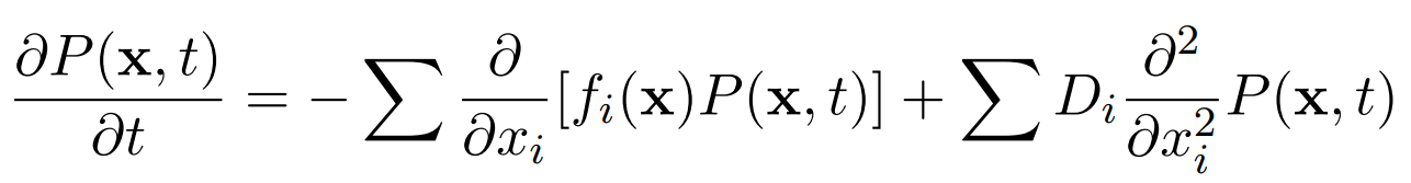
The Fokker-Planck equation is a partial differential equation for the probability density function $P(x,t)$:

$\frac{\partial P}{\partial t} = -\frac{\partial}{\partial x}[A(x,t)P] + \frac{\partial^2}{\partial x^2}[B(x,t)P]$

• $P(x,t)$ is the probability density of finding the system at state $x$ at time $t$
• $A(x,t)$ is the drift coefficient, encoding deterministic forces (systematic motion, potential gradients, external fields)
• $B(x,t)$ is the diffusion coefficient, encoding the strength of random fluctuations (related to temperature or noise intensity)

The first term on the right-hand side shifts the distribution (drift), while the second term spreads it out (diffusion). Both coefficients can depend on position and time, which allows for rich, nonlinear dynamics.

Physical Interpretation

Think of a cloud of probability density sitting on the $x$-axis. The drift term pushes that cloud in a preferred direction, like a current carrying it along. The diffusion term causes the cloud to spread, just as ink dropped in water disperses over time.

The Fokker-Planck equation captures the competition between these two effects. In many physical situations, drift tends to concentrate probability (e.g., a particle falling into a potential well), while diffusion tends to smear it out. The balance between them determines the shape of the steady-state distribution.

Probability Density Evolution

The equation tracks how the likelihood of finding a system in a given state changes moment by moment. From $P(x,t)$, you can compute any statistical quantity you need:

• Mean position: $\langle x \rangle = \int x \, P(x,t) \, dx$
• Variance: $\langle x^2 \rangle - \langle x \rangle^2$, which tells you how spread out the distribution is
• Higher moments for characterizing skewness, kurtosis, etc.

This makes the Fokker-Planck equation especially useful for studying relaxation processes, where a system starts in some non-equilibrium distribution and gradually approaches a steady state.

Mathematical Formulation

Drift and Diffusion Terms

The drift coefficient $A(x,t)$ captures all the systematic, predictable forces on the system. For a particle in a potential $V(x)$ with friction coefficient $\gamma$, the drift is typically $A(x) = -V'(x)/\gamma$. External fields or gradients also contribute here.

The diffusion coefficient $B(x,t)$ quantifies the intensity of random fluctuations. For thermal noise at temperature $T$ with friction $\gamma$, you often get $B = k_B T / \gamma$ from the fluctuation-dissipation relation. When $B$ depends on $x$, you need to be careful about the interpretation (Itô vs. Stratonovich), which affects the form of the equation.

Continuity Equation Connection

The Fokker-Planck equation is really a continuity equation for probability. Define the probability current:

$J(x,t) = A(x,t)P - \frac{\partial}{\partial x}[B(x,t)P]$

Then the Fokker-Planck equation becomes:

$\frac{\partial P}{\partial t} = -\frac{\partial J}{\partial x}$

This is the same structure as mass conservation in fluid dynamics. Total probability is conserved: it flows from one region of state space to another but never appears or disappears. At steady state, $\partial P / \partial t = 0$, so the current $J$ must be spatially uniform (and often zero for equilibrium systems, which is the condition of detailed balance).

Kramers-Moyal Expansion

The Fokker-Planck equation can be derived systematically from the master equation through the Kramers-Moyal expansion. Here's the logic:

1. Start with a master equation describing discrete transitions with rates $W(x'|x)$.

2. Taylor-expand the transition rates in the jump size $(x' - x)$.

3. This produces an infinite series of terms involving the $n$-th jump moments and $n$-th order spatial derivatives of $P$.

4. Truncate at second order. The first-order term gives drift; the second-order term gives diffusion.

The result is the standard Fokker-Planck equation. Higher-order terms capture non-Gaussian effects, but Pawula's theorem warns that truncating at any finite order above two can produce negative probabilities unless you keep all orders. In practice, the second-order truncation works well when individual jumps are small compared to the scale of variation in $P$.

Applications in Physics

Brownian Motion Modeling

Brownian motion is the classic application. A colloidal particle suspended in fluid experiences viscous drag (drift) and random bombardment by solvent molecules (diffusion). The Fokker-Planck equation for a free Brownian particle with diffusion constant $D$ is:

$\frac{\partial P}{\partial t} = D \frac{\partial^2 P}{\partial x^2}$

This is just the ordinary diffusion equation. Starting from a delta function at the origin, the solution is a Gaussian that broadens over time with mean square displacement $\langle x^2 \rangle = 2Dt$, recovering Einstein's 1905 result.

For a particle in a harmonic potential $V(x) = \frac{1}{2}kx^2$, the drift term pulls probability back toward the origin, and the steady-state solution is a Gaussian centered at $x = 0$ with width set by $k_BT/k$.

Stochastic Processes Description

Beyond Brownian motion, the Fokker-Planck framework applies to:

• Noise-induced transitions: Systems that hop between metastable states due to fluctuations (Kramers escape problem)
• Stochastic resonance: Weak periodic signals amplified by noise
• Financial modeling: The Black-Scholes equation for option pricing is structurally a Fokker-Planck equation
• Biological systems: Ion channel gating, molecular motor dynamics, and fluctuations in gene expression

Non-equilibrium Systems Analysis

The Fokker-Planck equation is particularly valuable for systems driven out of equilibrium by external forces, temperature gradients, or chemical potential differences. It can describe:

• Relaxation toward equilibrium and the timescales involved
• Non-equilibrium steady states where probability currents circulate without vanishing
• Transport phenomena under external driving (e.g., particles in a tilted periodic potential)
• Entropy production rates, which quantify how far a system is from equilibrium

Solution Methods

Analytical Approaches

Several techniques work depending on the structure of the problem:

1. Separation of variables: Write $P(x,t) = \sum_n c_n \phi_n(x) e^{-\lambda_n t}$. This works when $A$ and $B$ are time-independent, turning the PDE into an eigenvalue problem. The smallest nonzero eigenvalue $\lambda_1$ sets the longest relaxation time.
2. Transform methods: Fourier or Laplace transforms convert the PDE into an algebraic or ODE problem, especially useful for linear equations with constant coefficients.
3. Perturbation theory: For systems that are close to exactly solvable cases, expand the solution in a small parameter.
4. Similarity solutions: When the equation has scaling symmetry, you can reduce the PDE to an ODE using a similarity variable like $\eta = x / \sqrt{t}$.

Numerical Techniques

For problems without clean analytical solutions:

• Finite difference methods: Discretize space and time on a grid. The Crank-Nicolson scheme is popular for its stability and accuracy.
• Finite element methods: Better for complex geometries or spatially varying coefficients.
• Monte Carlo / stochastic simulation: Instead of solving the PDE directly, simulate many trajectories of the equivalent Langevin equation and build up $P(x,t)$ from histograms. Useful in high dimensions where grid-based methods become impractical.
• Spectral methods: Expand $P$ in a basis of orthogonal functions (Hermite polynomials for problems on $(-\infty, \infty)$, for example).

Boundary Conditions

The choice of boundary conditions depends on the physics:

• Reflecting ($J = 0$ at the boundary): No probability escapes. Models a hard wall or confinement.
• Absorbing ($P = 0$ at the boundary): Probability that reaches the boundary is removed. Models irreversible reactions or trapping.
• Periodic: $P$ and $J$ match at both ends of the interval. Used for angular variables or periodic potentials.
• Natural: $P$ and $J$ vanish as $x \to \pm\infty$. The standard choice for problems on the whole real line.

Relationship to Other Equations

Langevin Equation vs. Fokker-Planck

The Langevin equation describes a single stochastic trajectory:

$\frac{dx}{dt} = A(x,t) + \sqrt{2B(x,t)} \, \xi(t)$

where $\xi(t)$ is Gaussian white noise with $\langle \xi(t) \rangle = 0$ and $\langle \xi(t)\xi(t') \rangle = \delta(t - t')$.

The Fokker-Planck equation describes the probability distribution over all possible trajectories. These are two complementary views of the same physics: the Langevin picture is trajectory-by-trajectory, while the Fokker-Planck picture is ensemble-level. For Markovian processes with Gaussian noise, the two descriptions are exactly equivalent. You can derive the Fokker-Planck equation from the Langevin equation (and vice versa).

Master Equation Connection

The master equation governs transitions between discrete states:

$\frac{dP_n}{dt} = \sum_m [W_{nm}P_m - W_{mn}P_n]$

When the state space becomes continuous and individual jumps are small, a Taylor expansion of the master equation (the Kramers-Moyal expansion, truncated at second order) yields the Fokker-Planck equation. So the Fokker-Planck equation is the continuum, small-jump limit of the master equation. Both conserve total probability.

Kolmogorov Forward Equation

The Fokker-Planck equation is a special case of the Kolmogorov forward equation, which applies to general Markov processes, including those with discontinuous jumps. The Kolmogorov forward equation can include integral terms for jump processes (Lévy flights, for instance) that the standard Fokker-Planck equation doesn't capture. When the process is purely diffusive (no jumps), the Kolmogorov forward equation reduces to the Fokker-Planck form.

Extensions and Variations

Generalized Fokker-Planck Equation

The standard equation assumes local, Markovian dynamics. Generalizations relax these assumptions:

• Higher-order spatial derivatives capture non-Gaussian jump distributions
• Memory kernels replace instantaneous coefficients to model non-Markovian processes with temporal correlations
• Non-local spatial terms describe systems with long-range interactions

These generalizations are needed for anomalous diffusion, where $\langle x^2 \rangle$ doesn't grow linearly in time.

Non-linear Fokker-Planck Equations

In some systems, the drift or diffusion coefficients depend on $P$ itself, making the equation nonlinear. The Porous Medium Equation is one example. These arise in:

• Self-gravitating systems and mean-field models
• Crowd dynamics and collective motion
• Opinion formation models in sociophysics

Nonlinear Fokker-Planck equations can exhibit pattern formation, bistability, and other phenomena absent from the linear theory. They generally require numerical methods or special analytical techniques (e.g., self-similar solutions).

Fractional Fokker-Planck Equation

Replacing standard derivatives with fractional derivatives of order $\alpha$ models anomalous transport:

• Subdiffusion ($\langle x^2 \rangle \sim t^\alpha$ with $\alpha < 1$): Arises in crowded environments, disordered media, and viscoelastic materials. Modeled by a fractional time derivative.
• Superdiffusion ($\alpha > 1$): Arises from Lévy flights or active transport. Modeled by a fractional space derivative.

These equations connect to fractional calculus and are increasingly important in biophysics and materials science.

Statistical Mechanics Context

Ensemble Theory Connection

The Fokker-Planck equation describes probability evolution in the same spirit as the Liouville equation for Hamiltonian systems, but with dissipation and noise included. The Liouville equation conserves phase-space volume (no diffusion term), while the Fokker-Planck equation allows probability to spread and concentrate due to friction and fluctuations. This makes it the natural starting point for non-equilibrium ensemble theory.

Irreversibility and Entropy

The Fokker-Planck equation naturally produces irreversible dynamics. You can define a time-dependent entropy:

$S(t) = -\int P(x,t) \ln P(x,t) \, dx$

For systems relaxing toward equilibrium, $S(t)$ increases monotonically, connecting to the H-theorem and the second law of thermodynamics. The rate of entropy production can be expressed in terms of the probability current $J$, providing a quantitative measure of irreversibility.

Fluctuation-Dissipation Theorem

The fluctuation-dissipation theorem (FDT) states that the response of a near-equilibrium system to a small external perturbation is determined by its spontaneous equilibrium fluctuations. Within the Fokker-Planck framework, this connection emerges naturally: the drift coefficient (dissipation) and diffusion coefficient (fluctuations) are linked by

$B = \frac{k_B T}{\gamma}$

for a system at temperature $T$ with friction $\gamma$. This is the Einstein relation. The Fokker-Planck equation provides the machinery to derive and generalize the FDT, including extensions to non-equilibrium steady states.

Experimental Relevance

Diffusion Phenomena

The Fokker-Planck equation provides the theoretical backbone for interpreting diffusion experiments:

• Colloidal suspensions: Tracking particle positions over time and comparing to predicted $P(x,t)$
• Materials science: Diffusion of dopant atoms in semiconductors, described by position-dependent diffusion coefficients
• Anomalous diffusion: In biological cells, crowding by macromolecules produces subdiffusive behavior that requires fractional or generalized Fokker-Planck descriptions

Noise in Physical Systems

Noise is unavoidable in real experiments, and the Fokker-Planck equation provides the framework for analyzing it:

• Electronic noise: Johnson-Nyquist (thermal) noise and shot noise in circuits
• Mechanical oscillators: Thermal fluctuations of cantilevers in atomic force microscopy
• Laser physics: Intensity and phase fluctuations near threshold, where the Fokker-Planck equation for the electric field amplitude gives linewidth predictions

Chemical Reaction Kinetics

For reactions involving small numbers of molecules (e.g., inside a single cell), fluctuations matter and deterministic rate equations aren't sufficient. The Fokker-Planck equation describes:

• Fluctuations around the mean reaction trajectory
• Kramers escape rates: The rate at which a system crosses an energy barrier due to thermal noise, given by $k \sim \exp(-\Delta V / k_B T)$
• Stochastic gene expression, where transcription and translation involve small copy numbers and inherently noisy dynamics

Advanced Topics

Path Integral Formulation

The Fokker-Planck equation can be recast as a path integral (the Martin-Siggia-Rose or Onsager-Machlup formalism). The transition probability from state $x_0$ to $x_f$ in time $T$ is written as a sum over all paths, weighted by an "action" functional. This formulation:

• Connects directly to Feynman's path integrals in quantum mechanics
• Makes it natural to apply field-theoretic tools (saddle-point approximations, renormalization group)
• Is especially powerful for computing rare-event probabilities and large deviation functions

Quantum Fokker-Planck Equation

When a quantum system is coupled to a thermal environment, its reduced density matrix evolves according to a master equation that can sometimes be mapped onto a Fokker-Planck-like equation in phase space (using the Wigner function or P-representation). This describes:

• Decoherence and dissipation in open quantum systems
• Quantum-to-classical transitions
• Laser dynamics and quantum optical systems

The quantum version must respect the uncertainty principle, which constrains the minimum diffusion in phase space.

Fokker-Planck in Complex Systems

The formalism extends well beyond single-particle physics:

• Many-body systems: Coupled Fokker-Planck equations or high-dimensional single equations describe interacting agents or particles
• Biological networks: Gene regulatory networks, neural dynamics, and ecological models
• Non-equilibrium phase transitions: The Fokker-Planck equation near critical points reveals universal scaling behavior and critical slowing down

In these contexts, the main challenge is dimensionality. Analytical progress often requires mean-field approximations or projection onto low-dimensional order parameters.