5.1 Maxwell-Boltzmann distribution

Definition and importance

The Maxwell-Boltzmann distribution describes how particles in an ideal gas spread across different velocities and energies at thermal equilibrium. It connects the microscopic world of individual particle motion to macroscopic properties you can measure, like temperature and pressure.

This distribution is one of the most important results in classical statistical mechanics. It gives you a quantitative framework for predicting gas behavior, understanding chemical reaction rates, and calculating transport properties like diffusion and thermal conductivity.

Probability distribution function

The Maxwell-Boltzmann distribution is a probability density function that tells you the likelihood of finding a particle with a particular velocity or energy. It takes the form of an exponential decay weighted by the particle's kinetic energy relative to the thermal energy $kT$.

• Derived from statistical arguments about particle collisions and energy conservation
• Depends on three quantities: particle mass $m$, temperature $T$, and the Boltzmann constant $k$
• Applies to systems of distinguishable, non-interacting particles in thermal equilibrium

Role in classical statistical mechanics

The Maxwell-Boltzmann distribution serves as the foundation for much of classical thermal physics. From it, you can calculate average energies, pressures, and other thermodynamic quantities for gases. It also sets the stage for understanding quantum distributions (Fermi-Dirac and Bose-Einstein), which reduce to the Maxwell-Boltzmann form in the classical limit.

Beyond equilibrium properties, the distribution underpins the analysis of transport phenomena like diffusion and thermal conductivity in gases and liquids.

Derivation and assumptions

James Clerk Maxwell and Ludwig Boltzmann developed this distribution in the late 19th century, drawing on kinetic theory and probability theory. Their combined work established the statistical approach to thermodynamics that we still use today.

Maxwell's approach

Maxwell started by assuming that the three components of a particle's velocity ($v_x$, $v_y$, $v_z$) are statistically independent and that no direction in space is preferred (isotropy). From these two assumptions alone, he showed that the distribution for each velocity component must be a Gaussian. He also introduced the concept of the most probable speed and connected it to temperature.

Boltzmann's contribution

Boltzmann generalized Maxwell's velocity distribution to energy distributions and broader classes of systems. His key contributions include:

• The H-theorem, which explains why systems evolve toward equilibrium
• The concept of phase space and counting microstates
• The famous entropy formula $S = k \ln W$, relating entropy to the number of accessible microstates

Key assumptions and limitations

The derivation rests on several assumptions you should keep in mind:

• Particles are distinguishable and non-interacting (ideal gas approximation)
• The system is in thermal equilibrium
• Quantum effects are negligible (valid when the thermal de Broglie wavelength is much smaller than the average inter-particle spacing)
• External forces like gravity are neglected
• The distribution breaks down at very high densities or very low temperatures, where quantum statistics take over

Mathematical formulation

The distribution can be written in three related forms, depending on whether you're interested in velocity components, speed, or energy.

Velocity distribution

The full three-dimensional velocity distribution gives the probability density for a particle to have velocity $(v_x, v_y, v_z)$:

$f(v_x, v_y, v_z) = \left(\frac{m}{2\pi kT}\right)^{3/2} \exp\left(-\frac{m(v_x^2 + v_y^2 + v_z^2)}{2kT}\right)$

The prefactor $\left(\frac{m}{2\pi kT}\right)^{3/2}$ is the normalization constant, determined by requiring the total probability to equal 1. Notice the distribution has spherical symmetry in velocity space: it depends only on the magnitude of the velocity, not its direction.

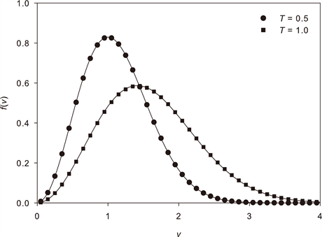
Speed distribution

To get the distribution of speeds (the magnitude $v = \sqrt{v_x^2 + v_y^2 + v_z^2}$), you integrate the velocity distribution over all directions. This introduces a factor of $4\pi v^2$ from the spherical shell volume element:

$f(v) = 4\pi v^2 \left(\frac{m}{2\pi kT}\right)^{3/2} \exp\left(-\frac{mv^2}{2kT}\right)$

The $v^2$ factor is crucial. It's why the speed distribution peaks at a nonzero value even though the velocity distribution peaks at zero: there are far more ways to have a large speed than a small one, because the spherical shell in velocity space grows as $v^2$.

Energy distribution

Using the substitution $E = \frac{1}{2}mv^2$ and the corresponding change of variables, the speed distribution transforms into an energy distribution:

$f(E) = \frac{2\pi}{(\pi kT)^{3/2}} \sqrt{E} \, \exp\left(-\frac{E}{kT}\right)$

This has two competing factors: the $\sqrt{E}$ term (density of states, which increases with energy) and the exponential decay $\exp(-E/kT)$ (Boltzmann factor, which suppresses high energies). Their competition produces a peak at a finite energy.

Properties and characteristics

Normalization condition

Every valid probability distribution must integrate to 1 over all possible values. For the speed distribution:

$\int_0^\infty f(v) \, dv = 1$

This condition is what fixes the normalization constant in each form of the distribution.

Most probable speed

The most probable speed $v_p$ is where the speed distribution $f(v)$ reaches its maximum. You find it by setting $\frac{df}{dv} = 0$:

$v_p = \sqrt{\frac{2kT}{m}}$

This is the speed you'd observe most frequently if you could measure individual particle speeds.

Average speed

The mean speed is the expectation value of $v$:

$\langle v \rangle = \int_0^\infty v \, f(v) \, dv = \sqrt{\frac{8kT}{\pi m}}$

It's slightly higher than $v_p$ because the distribution is asymmetric, with a long tail extending to high speeds that pulls the average upward.

Root mean square speed

The rms speed comes from the second moment of the distribution:

$v_{\text{rms}} = \sqrt{\langle v^2 \rangle} = \sqrt{\frac{3kT}{m}}$

This is directly tied to the average kinetic energy: $\langle E \rangle = \frac{1}{2}m v_{\text{rms}}^2 = \frac{3}{2}kT$. The ordering is always $v_p < \langle v \rangle < v_{\text{rms}}$, and all three scale as $\sqrt{T/m}$.

Applications and examples

Ideal gas behavior

The Maxwell-Boltzmann distribution provides the microscopic justification for ideal gas laws. By averaging over particle velocities, you can derive:

• The pressure-volume relationship (connecting molecular impacts on container walls to Boyle's law)
• The temperature dependence of gas properties like thermal expansion and heat capacity
• The equipartition result: each quadratic degree of freedom contributes $\frac{1}{2}kT$ to the average energy
• Properties of gas mixtures through partial pressures (Dalton's law)

Effusion and diffusion

The distribution directly predicts how fast gas escapes through a small hole (effusion). The effusion rate is proportional to $\langle v \rangle$, which goes as $1/\sqrt{m}$. This gives Graham's law: lighter molecules effuse faster in proportion to the inverse square root of their molar mass.

For diffusion, the distribution determines how quickly molecules spread through a medium. Diffusion coefficients depend on both temperature and molecular mass in ways predicted by the Maxwell-Boltzmann framework.

Chemical reaction rates

For a reaction to occur, colliding molecules typically need a minimum kinetic energy called the activation energy $E_a$. The fraction of molecules with energy above $E_a$ is approximately $\exp(-E_a / kT)$, which comes directly from the tail of the Maxwell-Boltzmann energy distribution.

This is the physical basis of the Arrhenius equation: $k = A \exp(-E_a / RT)$. As temperature increases, the tail of the distribution extends further, more molecules exceed the activation energy, and the reaction rate increases.

Relationship to other distributions

The Maxwell-Boltzmann distribution is the classical limit of the two quantum mechanical distributions. Understanding where it breaks down tells you when quantum statistics become necessary.

Maxwell-Boltzmann vs. Fermi-Dirac

The Fermi-Dirac distribution applies to fermions (particles with half-integer spin, like electrons). The Pauli exclusion principle forbids two fermions from occupying the same quantum state, which fundamentally changes the distribution at low temperatures or high densities.

• At high temperature and low density, Fermi-Dirac reduces to Maxwell-Boltzmann
• At low temperature, fermions fill states up to the Fermi energy, producing behavior completely unlike the classical prediction
• This distinction is essential for understanding electrons in metals and semiconductors

Maxwell-Boltzmann vs. Bose-Einstein

The Bose-Einstein distribution applies to bosons (particles with integer spin, like photons and phonons). Bosons can pile into the same quantum state, which leads to phenomena like Bose-Einstein condensation at very low temperatures.

• At high temperature and low density, Bose-Einstein also reduces to Maxwell-Boltzmann
• At low temperature, bosons cluster into the ground state, deviating sharply from classical predictions
• This is critical for understanding blackbody radiation, superfluidity, and laser physics

Experimental verification

Historical experiments

The first direct test came from Otto Stern's molecular beam experiment (1920), which measured the velocity distribution of silver atoms in vacuum and found agreement with the Maxwell-Boltzmann prediction. Earlier indirect support came from blackbody radiation measurements by Lummer and Pringsheim, and from Millikan's verification of the equipartition theorem through the oil drop experiment.

Modern validation techniques

• Laser spectroscopy provides high-resolution measurements of atomic and molecular velocity distributions through Doppler broadening analysis
• Neutron scattering probes energy distributions in condensed matter systems
• Ultracold atom experiments test the boundaries where Maxwell-Boltzmann statistics give way to quantum distributions
• Advanced statistical fitting techniques continue to confirm the distribution's accuracy across a wide range of conditions

Limitations and extensions

High density systems

At high densities, particles interact strongly and the ideal gas assumption fails. Corrections include:

• The van der Waals equation, which accounts for excluded volume and attractive interactions
• Virial expansions, which provide systematic corrections order by order in density
• Integral equation theories (like the Ornstein-Zernike equation) for describing liquids

Quantum effects

When the thermal de Broglie wavelength becomes comparable to the inter-particle spacing, quantum effects dominate and Maxwell-Boltzmann statistics fail. You then need Fermi-Dirac or Bose-Einstein statistics. Semiclassical methods like the Wigner function can bridge the gap between the classical and quantum regimes.

Non-equilibrium situations

The Maxwell-Boltzmann distribution strictly applies only at equilibrium. For systems out of equilibrium:

• The Boltzmann transport equation describes the evolution of the distribution function under external forces and collisions
• The BBGKY hierarchy and Langevin equation provide more general non-equilibrium frameworks
• The fluctuation-dissipation theorem connects equilibrium fluctuations to non-equilibrium response, linking the two regimes

Significance in thermodynamics

Connection to entropy

Boltzmann's H-theorem shows that a gas not yet in equilibrium will evolve toward the Maxwell-Boltzmann distribution, and that the entropy increases during this process. This provides a statistical interpretation of the second law of thermodynamics: systems evolve toward the macrostate with the largest number of microstates.

The connection is made precise by Boltzmann's entropy formula:

$S = k \ln W$

where $W$ is the number of microstates consistent with the macroscopic state.

Role in equipartition theorem

The Maxwell-Boltzmann distribution predicts that each quadratic term in the energy (each degree of freedom) contributes $\frac{1}{2}kT$ to the average energy. This equipartition theorem explains, for example, why the molar heat capacity of a monatomic ideal gas is $\frac{3}{2}R$ (three translational degrees of freedom).

Equipartition works well at high temperatures but fails at low temperatures, where quantum mechanics freezes out certain degrees of freedom. The Einstein and Debye models of solids were early quantum corrections that resolved the discrepancy between equipartition predictions and observed heat capacities.

Computational methods

Monte Carlo simulations

Monte Carlo methods use random sampling to generate particle configurations distributed according to the Maxwell-Boltzmann distribution. The Metropolis algorithm is particularly useful: it efficiently explores high-dimensional phase spaces by accepting or rejecting trial moves based on the Boltzmann factor $\exp(-\Delta E / kT)$.

These simulations can calculate thermodynamic averages, fluctuations, and phase behavior for systems ranging from simple gases to complex liquids and magnetic materials.

Molecular dynamics applications

Molecular dynamics (MD) simulates the time evolution of a system by numerically integrating Newton's equations of motion for each particle. In equilibrium, the trajectories naturally sample the Maxwell-Boltzmann distribution, allowing you to extract thermodynamic properties from time averages.

MD is especially powerful for studying transport properties (diffusion coefficients, viscosity), relaxation processes, and non-equilibrium phenomena. It's widely used in materials science, biophysics, and chemical engineering.