7.7 Stochastic processes

Stochastic processes provide the mathematical language for describing systems that evolve randomly over time. In non-equilibrium statistical mechanics, they're essential: they connect the microscopic randomness of individual particles to the macroscopic behavior we can measure, like diffusion coefficients or relaxation times.

This section covers the main types of stochastic processes, the mathematical tools used to analyze them, stochastic differential equations, and their applications in statistical mechanics and stochastic thermodynamics.

Fundamentals of stochastic processes

A stochastic process is a collection of random variables indexed by time (or space). Instead of predicting a single outcome, you track how a probability distribution evolves. This framework lets you describe systems where randomness is intrinsic, not just a nuisance to average away.

Definition and characteristics

A stochastic process $\{X(t)\}$ assigns a random variable to each value of a parameter $t$ (usually time). The key statistical properties that characterize a process are its mean, variance, and correlation structure.

Processes are classified along two axes:

• State space: discrete (e.g., number of molecules) or continuous (e.g., particle position)
• Time parameter: discrete (measurements at fixed intervals) or continuous (evolving at every instant)

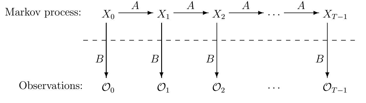
A particularly important property is the Markov property: the future state depends only on the present state, not on the history of how the system got there. Many processes in statistical mechanics are Markovian, which makes them far more tractable analytically.

Probability theory foundations

Stochastic processes are built on the axioms of probability:

• Non-negativity: $P(A) \geq 0$ for any event $A$
• Normalization: the total probability over the sample space equals 1
• Additivity: for mutually exclusive events, probabilities add

You'll also need conditional probability and Bayes' theorem for updating probabilities when new information arrives. Random variables are described by probability density functions (PDFs) in the continuous case and probability mass functions (PMFs) in the discrete case. The cumulative distribution function (CDF) gives the probability that the variable falls below a given value.

Random variables vs stochastic processes

A random variable captures the outcome of a single random experiment (e.g., the velocity of one particle at one instant). A stochastic process extends this to an entire trajectory: it's a function of time where each time slice is a random variable.

The crucial difference is that stochastic processes encode temporal correlations. Knowing $X(t_1)$ tells you something about $X(t_2)$, and quantifying that relationship is central to the analysis. Think of it this way: a single-day stock return is a random variable, but the full price history is a stochastic process.

Types of stochastic processes

Different physical phenomena call for different stochastic models. Choosing the right one depends on whether your system has discrete or continuous states, whether time is discrete or continuous, and what kind of noise drives the dynamics.

Discrete vs continuous time

• Discrete-time processes evolve at fixed intervals. They're naturally modeled with difference equations and arise when you sample a system at regular times (e.g., daily measurements).
• Continuous-time processes change at every instant. They're described by differential equations and are more natural for physical systems like radioactive decay or diffusion.

Sampling a continuous-time process at discrete intervals gives a discrete-time approximation, which is often how real data is collected.

Markov processes

Markov processes satisfy the memoryless property: $P(X(t_{n+1}) | X(t_n), X(t_{n-1}), \ldots) = P(X(t_{n+1}) | X(t_n))$. The entire future depends only on the present state.

This property makes them analytically tractable because you only need transition probabilities between states, not the full history. Markov processes include both discrete-time Markov chains and continuous-time variants. They're used extensively to model chemical reaction kinetics, population dynamics, and Monte Carlo sampling.

Poisson processes

The Poisson process models random events occurring at a constant average rate $\lambda$. Its defining features:

• Independent increments: events in non-overlapping time intervals are independent
• Stationary increments: the probability of $k$ events in an interval depends only on the interval length
• The number of events in time $t$ follows a Poisson distribution: $P(N=k) = \frac{(\lambda t)^k e^{-\lambda t}}{k!}$
• The time between successive events follows an exponential distribution with mean $1/\lambda$

Typical applications include radioactive decay, photon detection, and modeling rare events.

Wiener processes

The Wiener process (or standard Brownian motion) $W(t)$ is a continuous-time process with these properties:

• $W(0) = 0$
• Increments $W(t) - W(s)$ are Gaussian with mean 0 and variance $t - s$
• Increments over non-overlapping intervals are independent
• Sample paths are continuous but nowhere differentiable

This last point is physically significant: Brownian trajectories are extremely jagged at every scale. The Wiener process is the foundation for stochastic differential equations and appears throughout diffusion theory and financial modeling.

Mathematical tools for analysis

Probability distributions

Probability distributions describe the likelihood of different outcomes. Common ones in statistical mechanics:

• Discrete: binomial (fixed number of trials), Poisson (rare events at constant rate)
• Continuous: Gaussian/normal (central limit theorem), exponential (waiting times), Maxwell-Boltzmann (particle speeds)

For discrete variables, the PMF gives $P(X = x)$. For continuous variables, the PDF $f(x)$ gives probability density, so $P(a \leq X \leq b) = \int_a^b f(x)\,dx$. The CDF $F(x) = P(X \leq x)$ works for both.

Expectation and variance

The expectation (mean) of a random variable is its probability-weighted average:

$\langle X \rangle = \sum_i x_i P(x_i) \quad \text{(discrete)}, \qquad \langle X \rangle = \int x\, f(x)\, dx \quad \text{(continuous)}$

The variance measures the spread around the mean:

$\text{Var}(X) = \langle (X - \langle X \rangle)^2 \rangle = \langle X^2 \rangle - \langle X \rangle^2$

The standard deviation $\sigma = \sqrt{\text{Var}(X)}$ has the same units as $X$, making it more physically interpretable than the variance.

Autocorrelation functions

The autocorrelation function measures how correlated a process is with itself at a different time:

$C(\tau) = \langle X(t)\, X(t + \tau) \rangle$

For a stationary process, this depends only on the time lag $\tau$, not on $t$ itself. The rate at which $C(\tau)$ decays tells you the correlation time of the process, which is how quickly the system "forgets" its current state. A fast decay means short memory; a slow decay indicates long-range temporal correlations.

Autocorrelation functions are also used to detect hidden periodicities in noisy data.

Power spectral density

The power spectral density (PSD) $S(\omega)$ describes how the variance of a process is distributed across frequencies. It's computed as the Fourier transform of the autocorrelation function:

$S(\omega) = \int_{-\infty}^{\infty} C(\tau)\, e^{-i\omega\tau}\, d\tau$

This is the Wiener-Khinchin theorem. The PSD reveals dominant frequencies, periodic components, and noise characteristics. For example, white noise has a flat PSD (equal power at all frequencies), while $1/f$ noise has power concentrated at low frequencies.

Stochastic differential equations

Stochastic differential equations (SDEs) combine deterministic dynamics with random noise. They're the natural language for continuous-time stochastic models in physics, describing systems where both systematic forces and random fluctuations matter.

Langevin equation

The Langevin equation describes a particle subject to both deterministic and random forces:

$\frac{dx}{dt} = a(x, t) + b(x, t)\,\xi(t)$

Here $a(x, t)$ is the drift term (systematic force, like friction), $b(x, t)$ is the diffusion coefficient (noise amplitude), and $\xi(t)$ is white noise with $\langle \xi(t) \rangle = 0$ and $\langle \xi(t)\xi(t') \rangle = \delta(t - t')$.

For a Brownian particle with friction coefficient $\gamma$ in a potential, the Langevin equation directly connects the microscopic random kicks to the macroscopic damping. It serves as the starting point for most stochastic modeling in physics.

Fokker-Planck equation

While the Langevin equation tracks individual trajectories, the Fokker-Planck equation describes the time evolution of the probability density $P(x, t)$:

$\frac{\partial P}{\partial t} = -\frac{\partial}{\partial x}[a(x,t)\, P] + \frac{1}{2}\frac{\partial^2}{\partial x^2}[b^2(x,t)\, P]$

The first term on the right is the drift (probability flow due to systematic forces) and the second is the diffusion (spreading due to noise). The Fokker-Planck equation is equivalent to the Langevin equation but works at the level of distributions, making it useful for computing transition probabilities and stationary distributions.

Itô vs Stratonovich interpretations

When the noise coefficient $b(x, t)$ depends on $x$, you need to specify how to interpret the stochastic integral. The two standard choices are:

• Itô interpretation: evaluates $b(x, t)$ at the beginning of each time step. This leads to a modified chain rule called Itô's lemma, which differs from ordinary calculus.
• Stratonovich interpretation: evaluates $b(x, t)$ at the midpoint of each time step. The ordinary chain rule still applies, which often makes it more physically intuitive.

The two interpretations give different Fokker-Planck equations for the same Langevin equation when $b$ depends on $x$. The choice depends on the physics: Stratonovich is typically appropriate when the noise has a finite (but short) correlation time, while Itô arises naturally in certain mathematical contexts and in systems with truly delta-correlated noise.

Applications in statistical mechanics

Brownian motion

Brownian motion is the random motion of mesoscopic particles (like pollen grains) suspended in a fluid, caused by collisions with surrounding molecules. Einstein's 1905 analysis connected the diffusion coefficient $D$ to microscopic quantities via $D = k_B T / \gamma$, where $\gamma$ is the friction coefficient. This was one of the first direct confirmations of the molecular nature of matter.

Brownian motion is modeled by the Langevin equation or the Wiener process, and it remains central to studying colloidal suspensions, polymer dynamics, and molecular motors.

Diffusion processes

Diffusion describes the spreading of particles, heat, or other quantities through a medium. In the continuum limit, it's governed by Fick's second law:

$\frac{\partial c}{\partial t} = D\, \nabla^2 c$

where $c$ is concentration and $D$ is the diffusion coefficient. At the stochastic level, diffusion is described by the Fokker-Planck equation. The mean-squared displacement grows linearly with time: $\langle x^2 \rangle = 2Dt$ in one dimension. Deviations from this linear scaling indicate anomalous diffusion, which requires more advanced models.

Fluctuation-dissipation theorem

The fluctuation-dissipation theorem (FDT) connects a system's spontaneous fluctuations in equilibrium to its response to external perturbations. Concretely, it relates the autocorrelation function of equilibrium fluctuations to the linear response function (how the system responds to a small applied force).

This is profound: it means you can predict how a system will respond to a perturbation just by watching its equilibrium fluctuations. The FDT applies to electrical noise in resistors (Johnson-Nyquist noise), mechanical damping, and many other systems. It provides a direct bridge between equilibrium and near-equilibrium behavior.

Master equation

The master equation governs the time evolution of state probabilities in systems with discrete states:

$\frac{dP_i}{dt} = \sum_j \left[ W_{ij} P_j - W_{ji} P_i \right]$

Here $W_{ij}$ is the transition rate from state $j$ to state $i$. The first term represents probability flowing into state $i$; the second represents probability flowing out. At steady state, $dP_i/dt = 0$, and if detailed balance holds ($W_{ij}P_j = W_{ji}P_i$ for all pairs), the system is in thermodynamic equilibrium.

The master equation is used to model chemical reaction networks, population dynamics, and quantum open systems.

Numerical methods

Many stochastic problems can't be solved analytically. Numerical methods let you simulate trajectories, estimate distributions, and compute thermodynamic quantities for realistic models.

Monte Carlo simulations

Monte Carlo methods use random sampling to estimate quantities that are difficult to compute directly. In statistical mechanics, the Metropolis algorithm generates configurations sampled from the Boltzmann distribution $P \propto e^{-\beta E}$ without needing to enumerate all microstates.

The basic Metropolis steps:

1. Start from a configuration with energy $E_1$

2. Propose a random change to get a new configuration with energy $E_2$

3. If $E_2 < E_1$, accept the move

4. If $E_2 > E_1$, accept with probability $e^{-\beta(E_2 - E_1)}$

5. Repeat to generate a Markov chain of configurations

Monte Carlo is used to study phase transitions, critical phenomena, lattice models (like the Ising model), and protein folding.

Gillespie algorithm

The Gillespie algorithm (also called the stochastic simulation algorithm) generates exact trajectories for systems with discrete states and continuous time, particularly chemical reaction networks.

1. Calculate the propensity $a_j$ for each reaction $j$ (rate times the number of available reactant combinations)
2. Compute the total propensity $a_0 = \sum_j a_j$
3. Draw the time to the next reaction from an exponential distribution with rate $a_0$
4. Choose which reaction fires with probability $a_j / a_0$
5. Update the state and repeat

Unlike deterministic rate equations, the Gillespie algorithm captures stochastic fluctuations that matter in small systems, such as gene expression in individual cells.

Stochastic integration techniques

To numerically solve SDEs, you need specialized integrators that handle the noise term correctly:

• Euler-Maruyama method: the simplest scheme, analogous to Euler's method for ODEs but with an added noise increment $\Delta W \sim \mathcal{N}(0, \Delta t)$. It has strong order of convergence 0.5.
• Milstein method: adds a correction term that accounts for the noise-dependent part of the drift, achieving strong order 1.0.

Both methods require you to specify whether you're using Itô or Stratonovich calculus, since the discretization differs. Smaller time steps improve accuracy but increase computational cost.

Advanced concepts

Non-Markovian processes

Not all physical systems are memoryless. Non-Markovian processes have dynamics that depend on their history, not just the current state. This arises in systems with memory effects, such as:

• Particles in viscoelastic media, where the surrounding material has its own relaxation dynamics
• Glassy systems with slow, hierarchical relaxation
• Anomalous diffusion, where $\langle x^2 \rangle \sim t^\alpha$ with $\alpha \neq 1$

These processes are often modeled using generalized Langevin equations with memory kernels or fractional calculus. They're significantly harder to analyze than Markovian systems.

Lévy processes

Lévy processes generalize Brownian motion by allowing jumps (discontinuous paths) and heavy-tailed distributions. While the Wiener process has Gaussian increments with finite variance, Lévy processes can have stable distributions with infinite variance.

This means extreme events (large jumps) occur much more frequently than a Gaussian model would predict. Lévy processes are used to describe anomalous diffusion, turbulent transport, and financial market crashes. They're characterized by a Lévy-Khintchine formula that specifies the distribution of increments.

Fractional Brownian motion

Fractional Brownian motion (fBm) generalizes the Wiener process by introducing long-range correlations controlled by the Hurst exponent $H \in (0, 1)$:

• $H = 0.5$: standard Brownian motion (no correlations between increments)
• $H > 0.5$: persistent behavior (positive correlations; an upward trend tends to continue)
• $H < 0.5$: anti-persistent behavior (negative correlations; an upward trend tends to reverse)

Unlike standard Brownian motion, fBm is not Markovian (except at $H = 0.5$) and is not a semimartingale, which complicates its mathematical treatment. It's applied to turbulence, hydrology, financial time series, and network traffic modeling.

Stochastic thermodynamics

Stochastic thermodynamics extends the laws of thermodynamics to small systems where fluctuations are comparable to average values. At the nanoscale, the second law holds only on average: individual trajectories can transiently violate it.

Fluctuation theorems

Fluctuation theorems quantify the probability of observing "second-law-violating" trajectories. They state that while entropy-decreasing events can occur in small systems, they become exponentially unlikely as the system size or observation time increases.

These theorems are exact results, valid arbitrarily far from equilibrium. They include the Jarzynski equality and Crooks theorem as special cases, and they provide a statistical formulation of the second law.

Jarzynski equality

The Jarzynski equality relates the work done during a non-equilibrium process to the equilibrium free energy difference:

$\langle e^{-\beta W} \rangle = e^{-\beta \Delta F}$

Here $\beta = 1/(k_B T)$, $W$ is the work done on the system, and $\Delta F$ is the free energy difference between the final and initial equilibrium states. The angle brackets denote an average over many repetitions of the non-equilibrium protocol.

This is remarkable: you can extract equilibrium free energy differences from non-equilibrium measurements, no matter how far from equilibrium the process drives the system. It's been verified experimentally in single-molecule pulling experiments on RNA and DNA hairpins.

Crooks fluctuation theorem

The Crooks theorem relates the probability distributions of work in forward and time-reversed processes:

$\frac{P_F(W)}{P_R(-W)} = e^{\beta(W - \Delta F)}$

Here $P_F(W)$ is the probability of doing work $W$ in the forward process, and $P_R(-W)$ is the probability of doing work $-W$ in the reverse process. The Jarzynski equality can be derived from Crooks' theorem.

At the crossing point where $P_F(W) = P_R(-W)$, you get $W = \Delta F$, providing a practical method for estimating free energy differences. This has been applied to RNA folding/unfolding experiments and protein mechanics.