4.2 Double Integrals over General Regions

Understanding Double Integrals over General Regions

Double integrals over general regions let you integrate over shapes that aren't just rectangles. Instead of fixed constant limits on both integrals, at least one set of limits will be a function that traces the boundary of your region. This is how you actually compute areas, volumes, and physical quantities for real-world shapes like the region between two curves.

Setup of Double Integrals

Setting up the integral correctly is the hardest part. The computation itself is usually straightforward once the limits are right.

There are two types of general regions:

• Type I (vertical strips): The region is bounded between two functions of $x$. You integrate $y$ first (inner), then $x$ (outer). The outer limits on $x$ are constants, and the inner limits on $y$ are functions of $x$:

$\int_{a}^{b} \int_{g_1(x)}^{g_2(x)} f(x,y)\, dy\, dx$

• Type II (horizontal strips): The region is bounded between two functions of $y$. You integrate $x$ first (inner), then $y$ (outer). The outer limits on $y$ are constants, and the inner limits on $x$ are functions of $y$:

$\int_{c}^{d} \int_{h_1(y)}^{h_2(y)} f(x,y)\, dx\, dy$

The key rule: the outer integral always has constant limits, and the inner integral has variable limits that depend on the outer variable.

To set up a double integral over a general region:

1. Sketch the region and identify all boundary curves.
2. Decide whether Type I or Type II is simpler for the given region.
3. Write the outer limits as the constant range of the outer variable.
4. Express the inner limits as the lower and upper boundary functions in terms of the outer variable.
5. Evaluate the inner integral first, then the outer integral.

Sketching Integration Regions

A good sketch prevents most setup errors. Here's the process:

1. Plot each boundary curve on the coordinate plane (lines, parabolas, circles, etc.).
2. Find intersection points by solving the boundary equations simultaneously. These intersections determine where your limits change.
3. Shade the enclosed region.
4. Draw a representative strip through the region: a vertical strip if you're integrating $dy\, dx$, or a horizontal strip if you're integrating $dx\, dy$. The strip should enter the region at one boundary and exit at the other.

The strip tells you your inner limits. For a vertical strip, the bottom of the strip is $g_1(x)$ and the top is $g_2(x)$. For a horizontal strip, the left edge is $h_1(y)$ and the right edge is $h_2(y)$.

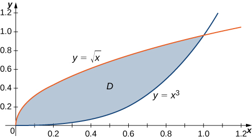
Example: For the region bounded by $y = x^2$ and $y = x + 2$, you'd find the intersections by solving $x^2 = x + 2$, giving $x = -1$ and $x = 2$. A vertical strip enters at $y = x^2$ (bottom) and exits at $y = x + 2$ (top), so the integral is:

$\int_{-1}^{2} \int_{x^2}^{x+2} f(x,y)\, dy\, dx$

Reversing Integration Order

Sometimes the integral is impossible (or very painful) to evaluate in one order but straightforward in the other. A classic example: $\int_0^1 \int_y^1 e^{x^2}\, dx\, dy$ can't be done inner-first because $e^{x^2}$ has no elementary antiderivative with respect to $x$. Switching the order makes it solvable.

To reverse the order:

1. Sketch the region from the original limits. Read the limits carefully to understand what shape they describe.
2. Re-describe the region using the other variable as the outer variable. Determine the constant range for the new outer variable, and express the new inner boundaries as functions of that variable.
3. Write the new integral with the swapped limits. The integrand $f(x,y)$ stays the same.

For the example above, the original limits describe the region where $0 \leq y \leq 1$ and $y \leq x \leq 1$. Sketching this gives a triangle. Re-describing with $x$ as the outer variable: $x$ ranges from $0$ to $1$, and for each $x$, $y$ ranges from $0$ to $x$. The reversed integral is:

$\int_0^1 \int_0^x e^{x^2}\, dy\, dx$

Now the inner integral with respect to $y$ is just $x e^{x^2}$, which you can integrate with a simple $u$-substitution.

Applications in Physics and Engineering

Once you can set up double integrals over general regions, a wide range of physical quantities become computable.

Area of a region: Integrate the constant function $f(x,y) = 1$ over the region. The double integral $\iint_R 1\, dA$ gives the area of $R$.

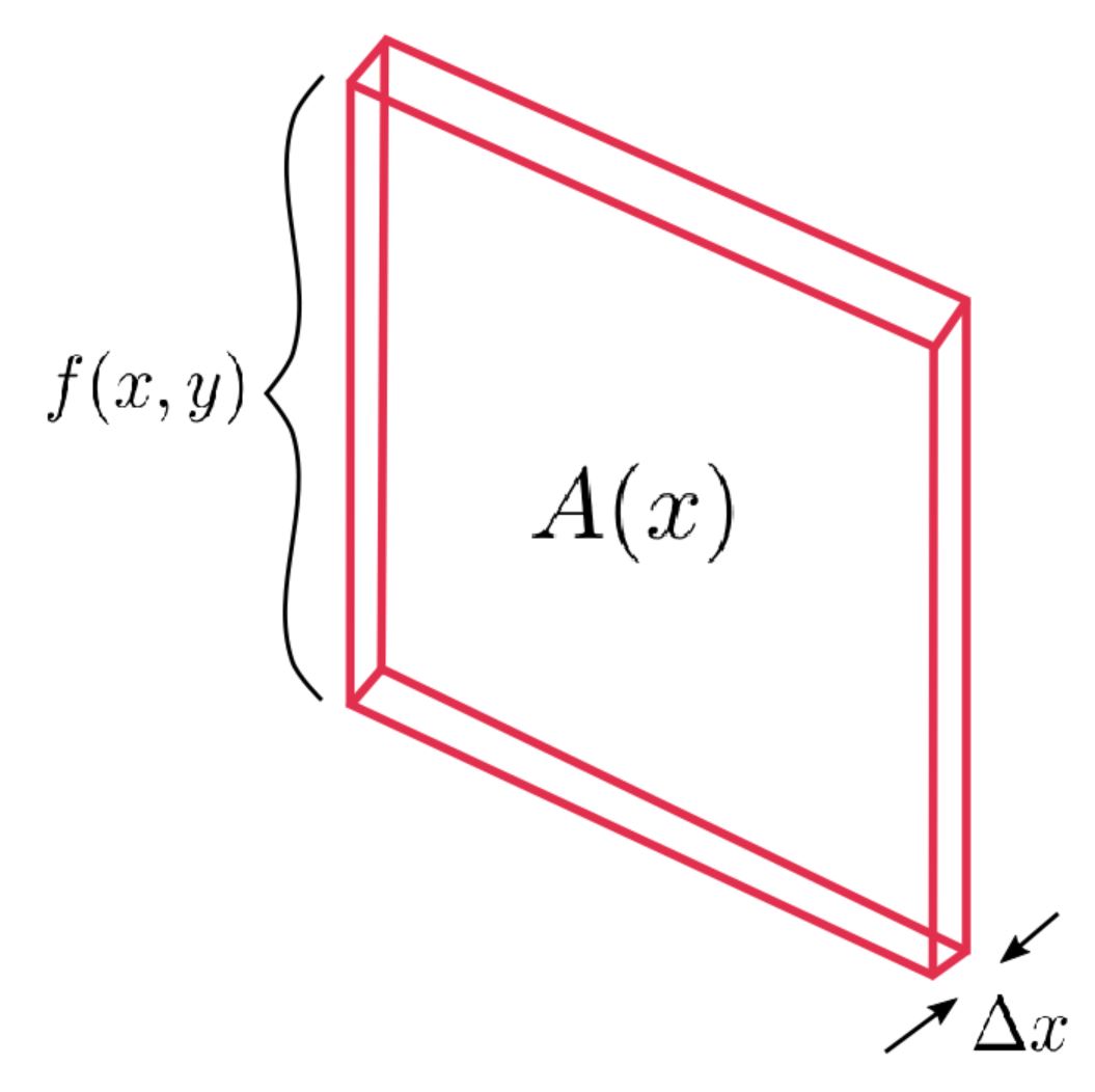
Volume under a surface: If $f(x,y) \geq 0$ over the region $R$, then $\iint_R f(x,y)\, dA$ gives the volume of the solid between $R$ and the surface $z = f(x,y)$. For instance, the volume under a paraboloid $z = 4 - x^2 - y^2$ over a disk can be computed this way.

Mass and center of mass: If a flat plate (lamina) has variable density $\rho(x,y)$, its total mass is $M = \iint_R \rho(x,y)\, dA$. The center of mass coordinates are:

$\bar{x} = \frac{1}{M}\iint_R x\,\rho(x,y)\, dA, \qquad \bar{y} = \frac{1}{M}\iint_R y\,\rho(x,y)\, dA$

Moments of inertia: The moment of inertia about the $x$-axis is $I_x = \iint_R y^2 \rho(x,y)\, dA$, and about the $y$-axis is $I_y = \iint_R x^2 \rho(x,y)\, dA$. These measure how the mass is distributed relative to each axis.

Other applications include computing fluid pressure on submerged surfaces (integrating depth times fluid density) and evaluating contributions to electric or gravitational fields by integrating over charge or mass distributions.