3.3 Partial Derivatives and the Gradient

Partial Derivatives

Partial derivatives of multivariable functions

A partial derivative measures how a function changes when you nudge one variable while freezing all the others. Think of it like asking: "If I only change $x$, how does the output respond?"

Notation: You'll see partial derivatives written several ways, all meaning the same thing:

$\frac{\partial f}{\partial x}, \quad f_x, \quad \frac{\partial f}{\partial y}, \quad f_y$

How to compute a partial derivative:

1. Pick the variable you're differentiating with respect to.
2. Treat every other variable as a constant.
3. Differentiate using the single-variable rules you already know.

Quick examples:

• $f(x,y) = x^2 y$: Taking $f_x$, treat $y$ as a constant. You get $f_x = 2xy$. For $f_y$, treat $x^2$ as a constant, giving $f_y = x^2$.
• $f(x,y) = \sin(xy)$: By the chain rule, $f_x = y\cos(xy)$ and $f_y = x\cos(xy)$.
• $f(x,y) = e^{x+y}$: Both partials give $e^{x+y}$, since the derivative of $x+y$ with respect to either variable is 1.

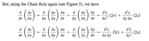
The chain rule extends naturally to partial derivatives for composite functions. If $f$ depends on $u$ and $v$, which themselves depend on $x$ and $y$, you chain the partials together. Implicit differentiation also carries over: if a relationship like $x^2 + y^2 + z^2 = 1$ defines $z$ implicitly, you can differentiate both sides with respect to $x$ (treating $z$ as a function of $x$) to find $\frac{\partial z}{\partial x}$.

Interpretation of partial derivatives

Geometrically, $f_x(a,b)$ is the slope of the tangent line to the surface $z = f(x,y)$ at the point $(a,b)$, sliced along the direction of the $x$-axis (with $y$ held fixed). Similarly, $f_y(a,b)$ gives the slope along the $y$-direction.

Partial derivatives connect directly to directional derivatives, which measure rates of change in any direction, not just along the coordinate axes.

Applications show up everywhere:

• Physics: Velocity components in 3D motion, where position depends on time and spatial coordinates.
• Economics: Marginal cost or marginal revenue, measuring how cost changes when you adjust one input (like labor) while holding others fixed.
• Sensitivity analysis: Determining which variable has the biggest impact on the output.

The linear approximation formula ties this together practically. For small changes $\Delta x$ and $\Delta y$:

$\Delta f \approx f_x \, \Delta x + f_y \, \Delta y$

This tells you that the total change in $f$ is approximately the sum of each partial derivative times the corresponding small change. It's the multivariable version of the single-variable approximation $\Delta f \approx f'(x)\Delta x$.

The Gradient and Higher-Order Derivatives

Higher-order partial derivatives

Just like in single-variable calculus, you can differentiate more than once. Second-order partial derivatives come in two flavors:

• Unmixed: Differentiate twice with respect to the same variable, e.g., $f_{xx} = \frac{\partial^2 f}{\partial x^2}$
• Mixed: Differentiate with respect to different variables, e.g., $f_{xy} = \frac{\partial^2 f}{\partial y \, \partial x}$ (differentiate first with respect to $x$, then $y$)

Clairaut's Theorem: If $f_{xy}$ and $f_{yx}$ are both continuous, then $f_{xy} = f_{yx}$. In practice, this holds for nearly every function you'll encounter in this course, so the order of mixed partials usually doesn't matter.

What second-order partials tell you:

• $f_{xx} > 0$ at a point means the function is concave up in the $x$-direction there; $f_{xx} < 0$ means concave down.
• Mixed partials $f_{xy}$ capture how the slope in one direction changes as you move in the other direction.
• These derivatives are essential for the second derivative test in optimization and for building Taylor series expansions of multivariable functions.

Gradient vector computation and geometry

The gradient packages all the partial derivatives of a function into a single vector:

$\nabla f = \left(\frac{\partial f}{\partial x}, \frac{\partial f}{\partial y}, \frac{\partial f}{\partial z}\right)$

For a function of two variables, drop the $z$-component.

Key properties of the gradient:

• It points in the direction of steepest ascent of $f$. If you're standing on a hillside and want to go uphill as fast as possible, walk in the direction of $\nabla f$.
• Its magnitude $\|\nabla f\|$ gives the rate of steepest ascent. A large magnitude means the function is changing rapidly.
• It is perpendicular to level curves (in 2D) and level surfaces (in 3D). This is why the gradient provides a normal vector to a surface at any point.

Connection to directional derivatives: The directional derivative of $f$ in the direction of a unit vector $\mathbf{u}$ is:

$D_{\mathbf{u}} f = \nabla f \cdot \mathbf{u}$

This dot product is maximized when $\mathbf{u}$ points in the same direction as $\nabla f$ (confirming the steepest ascent property) and equals zero when $\mathbf{u}$ is tangent to a level curve (no change along a contour).

Where the gradient shows up:

• Optimization: Setting $\nabla f = \mathbf{0}$ finds critical points where the function could have a maximum, minimum, or saddle point.
• Conservative vector fields: A vector field $\mathbf{F}$ is conservative if $\mathbf{F} = \nabla f$ for some scalar function $f$. One test for this is checking that the curl of $\mathbf{F}$ is zero.