4.4 Likelihood ratio tests

Definition of likelihood ratio

Likelihood ratio tests compare how well two competing statistical models explain the same observed data. By quantifying the relative support for each model, these tests give you a principled way to choose between hypotheses. In Bayesian statistics specifically, likelihood ratios serve as the engine that converts prior beliefs into posterior probabilities.

Likelihood function basics

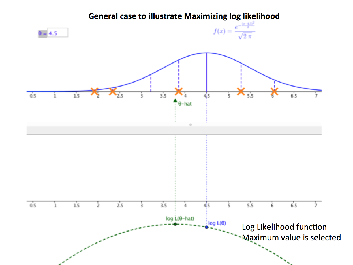
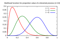
The likelihood function measures how well a statistical model explains observed data. It's calculated as the probability of observing your data given a specific set of parameter values:

$L(\theta|x) = P(x|\theta)$

Here, $\theta$ represents the model parameters and $x$ represents the observed data. The key idea: you hold the data fixed and vary the parameters, asking "which parameter values make this data most probable?" You then maximize this function to find the most likely parameter values for your dataset.

Ratio of likelihoods concept

Once you have likelihood values for two models, you compare them by forming a ratio:

$\Lambda = \frac{L(\theta_0|x)}{L(\theta_1|x)}$

where $\theta_0$ and $\theta_1$ are the parameter values under the null and alternative hypotheses, respectively. A ratio close to 1 means both models explain the data about equally well. A ratio much smaller than 1 means the alternative model fits substantially better. A ratio much larger than 1 favors the null.

Components of likelihood ratio test

A likelihood ratio test has several parts that work together: two competing hypotheses, a way to measure their relative fit, and a method for deciding whether the difference in fit is statistically meaningful.

Null hypothesis

The null hypothesis ($H_0$) represents the simpler, more restrictive model. It specifies a particular constraint on the model parameters, such as fixing a parameter to zero or requiring two parameters to be equal. This forms the baseline against which the alternative hypothesis is compared.

Alternative hypothesis

The alternative hypothesis ($H_1$ or $H_a$) represents the more complex, less restrictive model. It allows a broader range of parameter values. In a likelihood ratio test, the null model must be nested within the alternative model, meaning the null is a special case of the alternative with additional constraints imposed.

Note the nesting direction: the null hypothesis is nested within the alternative, not the other way around. The alternative includes all the parameters of the null plus additional ones (or relaxed constraints).

Test statistic calculation

The test statistic quantifies how much better the alternative model fits compared to the null. It's computed as:

$-2 \ln(\Lambda) = -2 \ln\left(\frac{L(\theta_0|x)}{L(\theta_1|x)}\right)$

Since the alternative model always fits at least as well as the null (it has more flexibility), $\Lambda \leq 1$, and the test statistic is always non-negative. Under certain regularity conditions, Wilks' theorem tells us this statistic approximately follows a chi-square distribution with degrees of freedom equal to the difference in the number of free parameters between the two models. Larger values indicate stronger evidence against the null.

Likelihood ratio test procedure

Step 1: Formulate hypotheses

• Define $H_0$ as the simpler model with parameter restrictions.
• Define $H_1$ as the more complex model without those restrictions.
• Make sure the null is nested within the alternative.
• Let your research question and prior knowledge guide which restrictions to test.

Step 2: Calculate likelihood values

• Fit both models using maximum likelihood estimation (MLE).
• Record the maximized likelihood for the null model: $L(\hat{\theta}_0|x)$.
• Record the maximized likelihood for the alternative model: $L(\hat{\theta}_1|x)$.

A practical note: you'll almost always work with log-likelihoods rather than raw likelihoods, since the raw values can be astronomically small numbers.

Step 3: Compute the test statistic

• Form the ratio: $\Lambda = \frac{L(\hat{\theta}_0|x)}{L(\hat{\theta}_1|x)}$
• Transform it: $-2 \ln(\Lambda) = -2[\ln L(\hat{\theta}_0|x) - \ln L(\hat{\theta}_1|x)]$
• The degrees of freedom equal the number of free parameters in the alternative model minus the number in the null model.
• For small samples, consider corrections like the Bartlett correction, since the chi-square approximation can be inaccurate.

Step 4: Determine the critical value and decide

• Choose a significance level $\alpha$ (commonly 0.05).
• Look up the critical value from a chi-square distribution with the appropriate degrees of freedom.
• If your test statistic exceeds the critical value, reject $H_0$. Otherwise, fail to reject it.

For example, with 2 degrees of freedom and $\alpha = 0.05$, the critical value is approximately 5.99. A test statistic of 8.3 would lead you to reject the null.

Interpretation of results

P-value approach

The p-value is the probability of getting a test statistic at least as extreme as the one you observed, assuming $H_0$ is true. You reject $H_0$ when the p-value falls below your chosen $\alpha$. Smaller p-values represent stronger evidence against the null, but remember that a p-value is not the probability that $H_0$ is true.

Critical value approach

This is the flip side of the p-value approach. You compare your test statistic directly to the predetermined critical value. If the statistic exceeds it, reject $H_0$. Both approaches always give the same decision for the same data and significance level.

Decision making process

• Weigh both statistical significance and practical importance. A statistically significant result can still be trivially small in real-world terms.
• Think about the costs of Type I errors (rejecting a true null) and Type II errors (failing to reject a false null). In some contexts, one type of error is far more costly than the other.
• Use the test result as one piece of evidence within a broader analysis, not as the final word.

Applications in Bayesian statistics

Model comparison

Likelihood ratios are central to comparing nested Bayesian models. The Bayesian counterpart of the likelihood ratio is the Bayes factor, which is the ratio of marginal likelihoods (likelihoods integrated over the prior) rather than maximized likelihoods. Likelihood ratio tests can also complement other model selection criteria like AIC and BIC, each of which penalizes model complexity differently.

Parameter estimation

Likelihood ratios help construct profile likelihood confidence intervals for individual parameters. In a Bayesian framework, you combine the likelihood with a prior distribution to get a posterior, and likelihood ratios can help you assess how much a specific parameter contributes to the model's fit.

Hypothesis testing

In Bayesian hypothesis testing, you multiply the likelihood ratio by the prior odds to get posterior odds. This is the core of Bayesian updating:

$\text{Posterior odds} = \text{Likelihood ratio} \times \text{Prior odds}$

This framework extends naturally to sequential testing, where you update your evidence as new data arrives.

Advantages and limitations

Strengths of likelihood ratio tests

• Provide a unified framework for comparing any pair of nested models.
• Handle complex hypotheses and model structures flexibly.
• Maintain good statistical power across a wide range of scenarios.
• Integrate naturally with Bayesian methods through Bayes factors.

Weaknesses and criticisms

• Rely on asymptotic (large-sample) approximations via Wilks' theorem, which can be inaccurate for small samples.
• Can be sensitive to model misspecification. If neither model is a good description of reality, the test may still confidently prefer one.
• Struggle with high-dimensional parameter spaces or irregular likelihood surfaces.
• Only apply directly to nested models. Comparing non-nested models requires different approaches (like Bayes factors or information criteria).

Likelihood ratio vs other tests

Three classical tests are asymptotically equivalent for testing parameter restrictions: the likelihood ratio test, the Wald test, and the score (Lagrange multiplier) test. They differ in what they require you to compute.

Wald test comparison

The Wald test only requires fitting the alternative (unrestricted) model. It uses the estimated parameter values and their standard errors to assess whether the restrictions implied by $H_0$ are consistent with the data. It's computationally simpler for large datasets, but it can behave poorly when the parameter estimates are far from the null values or when the sample is small. Likelihood ratio tests tend to be more reliable in those situations.

Score test comparison

The score test only requires fitting the null (restricted) model. It evaluates the slope of the log-likelihood at the null parameter values. If the slope is steep, the data are pulling the parameters away from the null, suggesting $H_0$ is wrong. Score tests can be more efficient when $H_0$ is true, while likelihood ratio tests tend to perform better when $H_1$ is true.

Bayesian extensions

Bayes factors

The Bayes factor is the Bayesian analog of the likelihood ratio, but it uses marginal likelihoods (the likelihood averaged over the prior) instead of maximized likelihoods:

$B_{10} = \frac{P(x|M_1)}{P(x|M_0)}$

where $M_1$ and $M_0$ are the alternative and null models. Jeffreys' scale provides rough guidelines for interpretation:

• $B_{10}$ between 1 and 3: barely worth mentioning
• $B_{10}$ between 3 and 10: moderate evidence for $M_1$
• $B_{10}$ between 10 and 30: strong evidence
• $B_{10}$ above 100: decisive evidence

Unlike classical likelihood ratio tests, Bayes factors automatically penalize model complexity through the prior, so they can compare non-nested models too.

Posterior odds ratio

The posterior odds combine the Bayes factor with your prior beliefs about which model is more plausible:

$\frac{P(M_1|x)}{P(M_0|x)} = B_{10} \times \frac{P(M_1)}{P(M_0)}$

This gives you a direct probability statement: "given the data and my priors, model $M_1$ is X times more probable than model $M_0$." If you start with equal prior odds ($P(M_1)/P(M_0) = 1$), the posterior odds equal the Bayes factor.

Computational considerations

Software implementations

• R: The lmtest package provides lrtest() for likelihood ratio tests. For Bayesian extensions, brms and rstanarm interface with Stan.
• Python: scipy.stats and statsmodels handle classical LR tests. PyMC and ArviZ support Bayesian model comparison.
• Dedicated Bayesian tools: Stan, JAGS, and BUGS allow flexible specification of models for computing marginal likelihoods and Bayes factors.

Numerical stability issues

Raw likelihoods involve products of many small probabilities, which can underflow to zero on a computer. Always work with log-likelihoods instead, turning products into sums. For matrix operations in multivariate models, Cholesky decomposition provides more stable computation than direct inversion. Regularization techniques can help when the likelihood surface is flat or poorly conditioned.

Real-world examples

Medical diagnosis applications

Likelihood ratios are a standard tool in diagnostic medicine. A positive likelihood ratio tells you how much more likely a positive test result is in someone with the disease versus someone without it. A negative likelihood ratio tells you the same for a negative result.

For instance, if a screening test has a positive likelihood ratio of 10, a positive result makes the disease 10 times more likely relative to the pre-test probability. Clinicians combine this with the patient's prior probability of disease (based on symptoms, demographics, etc.) to estimate the post-test probability using the posterior odds framework.

Financial modeling use cases

In finance, likelihood ratio tests help determine whether adding variables to a model meaningfully improves its explanatory power. For example, you might test whether adding a momentum factor to a three-factor asset pricing model significantly improves the fit. Bayesian model averaging, which weights models by their posterior probabilities (derived from Bayes factors), is used in portfolio optimization to account for model uncertainty rather than committing to a single "best" model.