Concept of Maximum Likelihood
Maximum likelihood estimation (MLE) is a method for estimating the parameters of a statistical model by finding the values that make your observed data most probable. It's one of the most widely used tools in frequentist statistics, but it also connects directly to Bayesian analysis since the likelihood function sits at the heart of both approaches.
Definition and Purpose
MLE answers a straightforward question: given the data you observed, which parameter values would have been most likely to produce it?
You start with a probability model (say, a normal distribution), observe some data, and then search for the parameter values (like the mean and variance) that maximize the probability of seeing that exact data. The resulting estimates have strong statistical properties:
- Consistency: as your sample size grows, the MLE converges to the true parameter value
- Asymptotic efficiency: among unbiased estimators, MLEs achieve the lowest possible variance (in large samples)
Historical Background
R.A. Fisher developed MLE in the 1920s as a principled alternative to older techniques like the method of moments and least squares. The approach gained traction in the mid-20th century as computational power made it practical to maximize complex likelihood functions. It also spawned related tools like likelihood ratio tests and information criteria (AIC, BIC).
Relationship to Bayesian Inference
This is where MLE becomes especially relevant for a Bayesian statistics course. The connection is direct:
- The likelihood function used in MLE is the same likelihood that appears in Bayes' theorem
- MLE is equivalent to finding the mode of the posterior when you use a flat (uniform) prior
- Bayesian methods treat parameters as random variables with distributions, while MLE treats them as fixed unknown quantities
- In practice, MLE often serves as a starting point or comparison benchmark for Bayesian models
The key difference: MLE gives you a single point estimate, while Bayesian inference gives you an entire posterior distribution over parameter values.
Likelihood Function
Mathematical Formulation
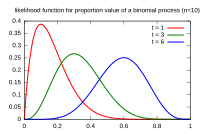
The likelihood function expresses how probable your observed data is for a given set of parameter values. It's written as:
where represents the parameters and represents the observed data. Numerically, this is the same as the probability (or density) function, but the perspective flips: the data is fixed, and you vary .
For independent and identically distributed (i.i.d.) observations, the likelihood factors into a product:
You use the probability density function (pdf) for continuous data or the probability mass function (pmf) for discrete data.
Properties of Likelihood
- The likelihood is not a probability distribution over . It doesn't integrate to 1 over the parameter space. This is a common point of confusion.
- It's invariant under one-to-one parameter transformations (if you reparameterize, the MLE transforms accordingly).
- The likelihood principle states that all the information the data provides about is contained in the likelihood function.
Log-Likelihood Function
In practice, you almost always work with the log-likelihood instead:
Why? Two reasons:
-
Products turn into sums, which are much easier to differentiate and compute:
-
Multiplying many small probabilities together causes numerical underflow on computers. Summing log-probabilities avoids this.
Because the logarithm is a strictly increasing function, maximizing the log-likelihood gives you the same answer as maximizing the likelihood itself.
Maximum Likelihood Estimators
Definition and Characteristics
The MLE is the parameter value that maximizes the likelihood (or equivalently, the log-likelihood):
A few things to keep in mind:
- MLEs are invariant under reparameterization: if is the MLE of , then is the MLE of for any one-to-one function
- MLEs don't always exist (the likelihood might not have a finite maximum), and they aren't always unique
Asymptotic Properties
As the sample size grows large, MLEs have three key properties under standard regularity conditions:
- Consistency: as
- Asymptotic normality: the distribution of approaches a normal distribution centered at the true value
- Asymptotic efficiency: the variance approaches the Cramér-Rao lower bound, meaning no unbiased estimator can do better
Formally, for large :
where is the Fisher information. The convergence rate is . These asymptotic results are the basis for constructing confidence intervals and hypothesis tests from MLEs.
Methods for Finding MLEs
Analytical Solutions
For some distributions, you can solve for the MLE by hand:
- Write down the log-likelihood
- Take the derivative with respect to and set it equal to zero:
- Solve for
- Verify it's a maximum (check the second derivative is negative)
Example (Normal distribution): For data drawn from , the MLEs are the sample mean and the sample variance . (Note: this MLE for variance divides by , not , so it's slightly biased in small samples.)
Closed-form solutions also exist for exponential and Poisson distributions, among others.
Numerical Optimization Techniques
Most real-world models don't have neat closed-form MLEs. In those cases, you use iterative algorithms:
- Newton-Raphson: uses both the gradient and the Hessian (second derivative matrix) to take smart steps toward the maximum. Fast convergence near the solution.
- Gradient descent/ascent: follows the slope of the log-likelihood uphill. Simpler but can be slower.
- Quasi-Newton methods (like BFGS): approximate the Hessian to reduce computation per step.
These methods require you to choose starting values carefully. Poor starting points can lead to convergence at a local maximum rather than the global one, or failure to converge at all.
EM Algorithm
The Expectation-Maximization (EM) algorithm handles models with latent (hidden) variables or missing data:
- E-step: Compute the expected value of the log-likelihood, averaging over the latent variables using current parameter estimates
- M-step: Maximize that expected log-likelihood to get updated parameter estimates
- Repeat until the estimates stabilize (converge)
The EM algorithm guarantees the likelihood increases at every iteration, but it can get stuck at local maxima. It's widely used for mixture models, hidden Markov models, and factor analysis.
Applications in Statistical Models
Linear Regression
Under the assumption of normally distributed errors with constant variance, the MLEs for regression coefficients are identical to the ordinary least squares (OLS) estimates:
This is one of the rare cases with a clean closed-form solution. The MLE framework adds a probabilistic interpretation to what's otherwise a purely algebraic fitting procedure.
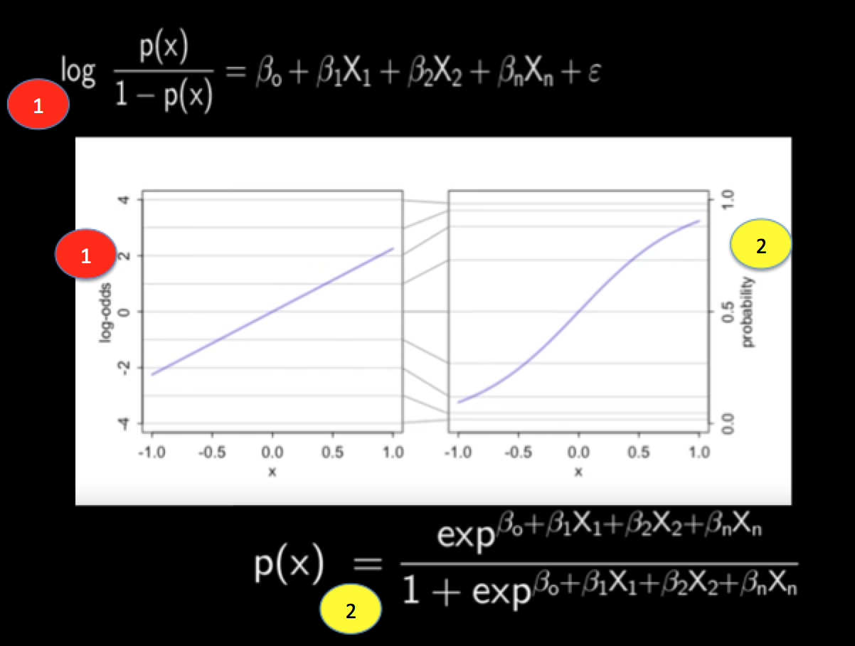
Logistic Regression
For binary outcomes (0/1), logistic regression models the probability of success using the logistic function. Each observation follows a Bernoulli distribution, so the log-likelihood is:
where . There's no closed-form solution here because of the nonlinearity, so MLEs are found through iterative methods like Newton-Raphson or iteratively reweighted least squares (IRLS).
Poisson Regression
Poisson regression models count data (number of events) using a log-link function to keep predicted values non-negative. MLEs are found numerically. Common applications include modeling accident rates, disease counts, or species abundance.
Likelihood Ratio Tests
Test Statistic Formulation
Likelihood ratio tests compare how well two models explain the data. The test statistic is:
where is the parameter value under the null hypothesis and is the unrestricted MLE. Larger values of mean the data are much more probable under the alternative than under the null.
Asymptotic Distribution
Under the null hypothesis and standard regularity conditions, follows a chi-squared distribution as the sample size grows:
where is the difference in the number of free parameters between the two models. This result lets you compute p-values and critical values for hypothesis testing.
Power of Likelihood Ratio Tests
The power of a test is the probability of correctly rejecting a false null hypothesis. For likelihood ratio tests:
- Power increases with sample size and effect size
- In finite samples, likelihood ratio tests are often more powerful than alternatives like the Wald test or score test
- For complex models, power can be estimated through simulation
Limitations and Alternatives
Small Sample Issues
The appealing asymptotic properties of MLEs (consistency, efficiency, normality) rely on large samples. In small samples:
- MLEs can be biased (recall the vs. issue for variance)
- Confidence intervals based on asymptotic normality may have poor coverage
- Bayesian methods with informative priors often produce more stable and reliable estimates when data is scarce
Regularization Techniques
In high-dimensional settings (many parameters relative to observations), MLEs tend to overfit. Regularization adds a penalty to the likelihood to constrain parameter estimates:
- Ridge regression (L2 penalty): shrinks coefficients toward zero
- Lasso (L1 penalty): shrinks some coefficients exactly to zero, performing variable selection
- Elastic net: combines L1 and L2 penalties
These methods trade a small amount of bias for a large reduction in variance.
Bayesian vs. Maximum Likelihood
| MLE | Bayesian | |
|---|---|---|
| Parameters | Fixed unknown quantities | Random variables with distributions |
| Prior information | Not used | Incorporated via prior |
| Output | Point estimate (+ confidence intervals) | Full posterior distribution |
| Small samples | Can be unreliable | Priors stabilize estimates |
| Computation | Often simpler | Can be more demanding (MCMC) |
MLE can be viewed as the Bayesian MAP (maximum a posteriori) estimate with a uniform prior. In large samples, the two approaches typically agree closely because the likelihood dominates the prior.
Computational Aspects
Software Implementations
- R:
optim(),nlm(),glm(), and thebbmlepackage - Python:
scipy.optimize,statsmodels,scikit-learn - Bayesian tools like Stan and PyMC often use MLE as a starting point for MCMC sampling
Computational Complexity
Complexity depends heavily on the model. Simple distributions with closed-form MLEs are trivial to compute. Iterative methods for complex models may require many evaluations of the likelihood and its derivatives, and high-dimensional problems can become computationally expensive.
Parallel Processing
Because the likelihood for i.i.d. data is a product (or sum of logs) over independent observations, likelihood evaluations are naturally parallelizable. This is especially useful for bootstrap resampling and cross-validation on large datasets.
Advanced Topics
Profile Likelihood
When your model has nuisance parameters (parameters you need but don't care about), the profile likelihood lets you focus on the parameter of interest. For each candidate value of that parameter, you maximize the likelihood over all the nuisance parameters. The resulting curve gives you a likelihood that depends only on the parameter you care about, which is useful for constructing confidence intervals in complex models.
Penalized Maximum Likelihood
This generalizes regularization within the likelihood framework. You maximize:
where is a penalty function (L1, L2, or something else) and controls the strength of penalization. This connects naturally to Bayesian inference: an L2 penalty corresponds to a Gaussian prior on the parameters, and an L1 penalty corresponds to a Laplace prior.
Empirical Likelihood Methods
Empirical likelihood is a nonparametric approach that constructs a likelihood function without assuming a specific distributional form. It combines the flexibility of nonparametric statistics with the inferential power of likelihood-based methods, and it's used for constructing confidence regions and hypothesis tests in semiparametric models.