3.4 Jeffreys priors

Jeffreys priors are a key tool in Bayesian statistics, providing a method for selecting prior distributions when little is known about parameters. They connect information theory and Bayesian inference, enhancing objectivity in statistical analyses.

These priors remain unchanged under reparameterization, allowing data to dominate inference. Defined using the Fisher information matrix, Jeffreys priors address the need for objective methods in statistical analysis and have influenced the development of other noninformative priors.

Definition of Jeffreys priors

• Jeffreys priors serve as a cornerstone in Bayesian statistics providing a method for selecting prior distributions
• These priors play a crucial role in situations where little or no prior information exists about the parameters of interest
• Jeffreys priors connect the concepts of information theory and Bayesian inference enhancing the objectivity of statistical analyses

Invariance property

Top images from around the web for Invariance property

• 

  Bayesian Probability Illustration Diagram | TikZ example View original

  Is this image relevant?

• 

  Frontiers | Dangers of the Defaults: A Tutorial on the Impact of Default Priors When Using ... View original

  Is this image relevant?

• 

  neuroscicomplab: Bayesianische Statistik View original

  Is this image relevant?

• 

  Bayesian Probability Illustration Diagram | TikZ example View original

  Is this image relevant?

• 

  Frontiers | Dangers of the Defaults: A Tutorial on the Impact of Default Priors When Using ... View original

  Is this image relevant?

1 of 3

Top images from around the web for Invariance property

• 

  Bayesian Probability Illustration Diagram | TikZ example View original

  Is this image relevant?

• 

  Frontiers | Dangers of the Defaults: A Tutorial on the Impact of Default Priors When Using ... View original

  Is this image relevant?

• 

  neuroscicomplab: Bayesianische Statistik View original

  Is this image relevant?

• 

  Bayesian Probability Illustration Diagram | TikZ example View original

  Is this image relevant?

• 

  Frontiers | Dangers of the Defaults: A Tutorial on the Impact of Default Priors When Using ... View original

  Is this image relevant?

1 of 3

• Remains unchanged under reparameterization of the model
• Preserves the same information regardless of how parameters are expressed
• Ensures consistency in inference across different parameterizations
• Applies to both continuous and discrete parameter spaces

Noninformative nature

• Designed to have minimal impact on the posterior distribution
• Allows the data to dominate the inference process
• Represents a state of ignorance about the parameter values
• Often results in flat or diffuse distributions over the parameter space

Mathematical formulation

• Defined as the square root of the determinant of the Fisher information matrix
• Expressed mathematically as $p(\theta) \propto \sqrt{|I(\theta)|}$
• $I(\theta)$ represents the Fisher information matrix
• Captures the curvature of the log-likelihood function
• Generalizes to multiple parameters through the use of the matrix determinant

Historical context

• Jeffreys priors emerged as a solution to the problem of prior selection in Bayesian inference
• These priors addressed the need for objective methods in statistical analysis
• Development of Jeffreys priors coincided with the broader formalization of Bayesian statistics

Harold Jeffreys' contribution

• Introduced the concept in his 1939 book "Theory of Probability"
• Sought to create a systematic method for choosing prior distributions
• Emphasized the importance of invariance in statistical inference
• Laid the groundwork for modern objective Bayesian methods

Development in Bayesian theory

• Sparked debates about the nature of objectivity in statistics
• Influenced the development of other noninformative priors (reference priors)
• Led to advancements in hierarchical Bayesian modeling
• Contributed to the broader acceptance of Bayesian methods in various scientific fields

Derivation of Jeffreys priors

• Jeffreys priors derive from the principle of maximizing the expected information gain
• These priors incorporate the model structure into the prior selection process
• Derivation involves concepts from information theory and differential geometry

Fisher information matrix

• Measures the amount of information a random variable carries about an unknown parameter
• Defined as the negative expected value of the second derivative of the log-likelihood function
• Expressed mathematically as $I(\theta) = -E[\frac{\partial^2}{\partial\theta^2} \log f(x|\theta)]$
• Captures the curvature of the log-likelihood function around the true parameter value

Square root of determinant

• Taking the square root of the determinant ensures proper scaling
• Produces a prior that is invariant under reparameterization
• Results in a prior that is proportional to the volume element in the parameter space
• Generalizes the concept of "flatness" to multidimensional parameter spaces

Multivariate extension

• Extends the concept to models with multiple parameters
• Uses the full Fisher information matrix instead of a single value
• Accounts for potential correlations between parameters
• Requires careful consideration of parameter interactions and constraints

Properties of Jeffreys priors

• Jeffreys priors possess unique characteristics that make them valuable in Bayesian inference
• These properties ensure consistency and objectivity in statistical analyses
• Understanding these properties helps in appropriate application of Jeffreys priors

Reparameterization invariance

• Remains unchanged under one-to-one transformations of parameters
• Ensures consistent inference regardless of the chosen parameterization
• Preserves the geometric structure of the parameter space
• Particularly useful when dealing with non-linear models

Consistency under marginalization

• Maintains coherence when reducing the dimensionality of the parameter space
• Allows for consistent inference on subsets of parameters
• Supports hierarchical modeling and partial inference scenarios
• Facilitates modular approach to complex statistical problems

Improper prior distributions

• Often results in improper priors that do not integrate to a finite value
• Requires careful consideration to ensure proper posterior distributions
• Can lead to issues in model comparison and Bayes factor calculations
• Necessitates the use of techniques like posterior propriety checks

Applications in Bayesian inference

• Jeffreys priors find wide application across various domains of Bayesian statistics
• These priors provide a starting point for many statistical analyses
• Application varies depending on the nature of the parameters being estimated

Location parameters

• Used for parameters that shift the probability distribution (mean)
• Often results in uniform priors for location parameters
• Facilitates inference in models with unknown central tendencies
• Applies to various distributions (normal, Cauchy, logistic)

Scale parameters

• Employed for parameters that stretch or shrink the distribution (variance)
• Typically leads to priors proportional to 1/σ for scale parameters
• Supports inference in heteroscedastic models
• Relevant for distributions like gamma, exponential, and Weibull

Shape parameters

• Utilized for parameters that affect the shape of the distribution (skewness, kurtosis)
• Often results in more complex prior forms
• Facilitates inference in flexible distribution families (beta, gamma)
• Requires careful consideration of parameter constraints and interpretability

Advantages of Jeffreys priors

• Jeffreys priors offer several benefits in Bayesian analysis enhancing the robustness and objectivity of statistical inferences
• These advantages make Jeffreys priors a popular choice in many applications
• Understanding these benefits helps in deciding when to use Jeffreys priors

Objectivity in prior selection

• Provides a systematic approach to choosing priors without subjective input
• Reduces the potential for bias in the analysis
• Allows for consistent results across different researchers
• Particularly useful in scientific studies where objectivity is crucial

Automatic prior generation

• Derives the prior directly from the likelihood function
• Eliminates the need for manual specification of prior distributions
• Facilitates automated Bayesian analysis in complex models
• Supports reproducibility in statistical research

Invariance to transformations

• Maintains consistency under different parameterizations of the model
• Ensures that inferences are not affected by arbitrary choices of scale or units
• Supports the principle of scientific invariance
• Particularly valuable in physics and engineering applications

Limitations and criticisms

• Despite their advantages Jeffreys priors face several challenges and criticisms
• Understanding these limitations helps in appropriate application and interpretation of results
• These issues have led to ongoing research and development of alternative approaches

Computational complexity

• Can be difficult to derive analytically for complex models
• Often requires numerical approximation methods
• May lead to increased computational time in high-dimensional problems
• Necessitates the use of advanced computational techniques (MCMC)

Improper posteriors

• Sometimes results in improper posterior distributions
• Can lead to issues in model comparison and hypothesis testing
• Requires careful verification of posterior propriety
• May necessitate the use of alternative priors in some cases

Jeffreys-Lindley paradox

• Occurs in hypothesis testing scenarios with point null hypotheses
• Can lead to inconsistent results as sample size increases
• Challenges the interpretation of Bayes factors with Jeffreys priors
• Has sparked debates about the nature of Bayesian hypothesis testing

Comparison with other priors

• Comparing Jeffreys priors with other prior choices provides insights into their strengths and weaknesses
• This comparison helps in selecting the most appropriate prior for a given problem
• Understanding these differences aids in interpreting results from different Bayesian analyses

Jeffreys vs uniform priors

• Jeffreys priors are invariant under reparameterization unlike uniform priors
• Uniform priors can lead to paradoxical results in some cases (Bertrand's paradox)
• Jeffreys priors often provide more consistent results across different parameterizations
• Uniform priors may be simpler to implement and interpret in some scenarios

Jeffreys vs reference priors

• Reference priors aim to maximize the expected Kullback-Leibler divergence
• Jeffreys priors are a special case of reference priors for single-parameter models
• Reference priors can be more appropriate for multi-parameter problems
• Jeffreys priors are often simpler to derive and implement

Jeffreys vs maximum entropy priors

• Maximum entropy priors maximize uncertainty given constraints
• Jeffreys priors focus on invariance and information content
• Maximum entropy priors can incorporate prior knowledge more explicitly
• Jeffreys priors are often more generally applicable across different model types

Examples and case studies

• Examining specific examples helps in understanding the application of Jeffreys priors
• These case studies illustrate the derivation and use of Jeffreys priors in practice
• Studying these examples provides insights into the behavior of Jeffreys priors in different scenarios

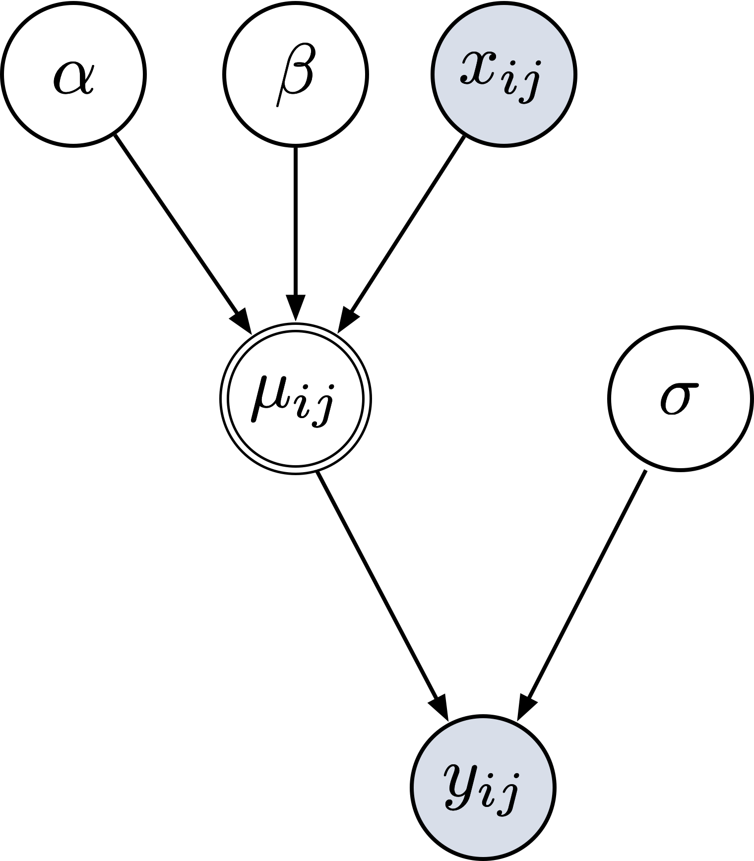
Normal distribution

• Jeffreys prior for the mean (μ) is uniform
• Prior for the standard deviation (σ) is proportional to 1/σ
• Joint prior for (μ, σ) is p(μ, σ) ∝ 1/σ²
• Demonstrates how Jeffreys priors handle location and scale parameters

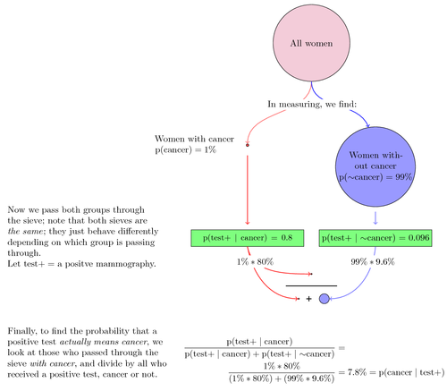
Binomial distribution

• Jeffreys prior for the success probability (p) is Beta(1/2, 1/2)
• Equivalent to the arcsine distribution
• Puts more weight on probabilities near 0 and 1 compared to a uniform prior
• Illustrates how Jeffreys priors behave for bounded parameters

Poisson distribution

• Jeffreys prior for the rate parameter (λ) is proportional to 1/√λ
• Improper prior that requires careful handling
• Demonstrates how Jeffreys priors deal with non-negative parameters
• Highlights the need for posterior propriety checks

Practical implementation

• Implementing Jeffreys priors in practice involves several considerations and techniques
• These practical aspects are crucial for effective use of Jeffreys priors in real-world problems
• Understanding these implementation details helps in conducting robust Bayesian analyses

Numerical approximation methods

• Often necessary for complex models where analytical solutions are intractable
• Includes techniques like quadrature methods for low-dimensional problems
• Employs Monte Carlo integration for higher-dimensional cases
• May require adaptive algorithms to handle varying scales and shapes of priors

Software tools for Jeffreys priors

• Several statistical software packages support the use of Jeffreys priors
• Popular tools include Stan, PyMC, and JAGS for Bayesian modeling
• Some packages offer built-in functions for common Jeffreys priors
• Custom implementation may be necessary for specialized models

Diagnostic checks

• Crucial for ensuring the validity of results when using Jeffreys priors
• Includes checks for posterior propriety and convergence of MCMC algorithms
• Involves sensitivity analyses to assess the impact of prior choice
• May require comparison with other prior choices for robustness

Advanced topics

• Jeffreys priors extend beyond basic applications into more complex statistical scenarios
• These advanced topics represent areas of ongoing research and development
• Understanding these concepts provides insights into the frontiers of Bayesian statistics

Jeffreys priors for hierarchical models

• Extends the concept to multi-level models with nested parameters
• Requires careful consideration of the hierarchical structure
• May involve partial pooling of information across levels
• Presents challenges in terms of interpretation and computation

Mixture of Jeffreys priors

• Combines multiple Jeffreys priors to handle complex parameter spaces
• Useful for models with different types of parameters (location, scale, shape)
• Can provide more flexibility in prior specification
• Requires careful consideration of the mixing proportions

Modifications for specific problems

• Tailors Jeffreys priors to address specific issues or incorporate additional information
• Includes techniques like regularization to handle high-dimensional problems
• May involve combining Jeffreys priors with informative priors
• Represents an active area of research in Bayesian methodology