Highest posterior density (HPD) regions identify the most probable values of a parameter given observed data. They give you the smallest possible region of parameter space that contains a specified amount of posterior probability, making them one of the most efficient summaries of a posterior distribution.
Unlike equal-tailed credible intervals, HPD regions can be asymmetric or even disjoint. This flexibility lets them faithfully reflect the actual shape of the posterior, which matters most when you're working with skewed or multimodal distributions.
Definition of HPD regions
An HPD region is a subset of the parameter space where every point inside the region has a higher posterior density than every point outside it, and the region contains a specified total probability (say, 95%). Think of it as drawing a horizontal line across the density curve and collecting everything above that line. You raise or lower the line until the area under the curve in that collected region equals your target probability.
Concept of posterior density
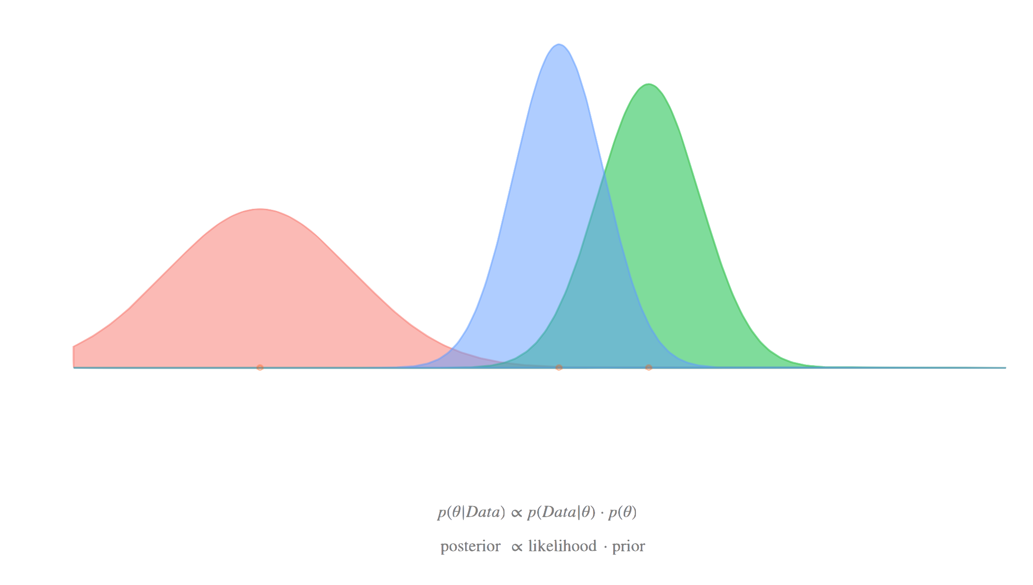
The posterior density describes how probable each parameter value is after you've observed data . It combines your prior beliefs with the likelihood of the data through Bayes' theorem:
You can visualize it as a curve (for one parameter) or a surface (for two parameters), where taller regions correspond to more probable parameter values. The HPD region is built directly from this curve.
Characteristics of HPD regions
- Every point inside the region has a posterior density at least as high as every point outside it
- For a given probability content (e.g., 95%), the HPD region has the smallest possible volume of any credible region
- The region always contains the posterior mode (the peak of the distribution)
- For multimodal posteriors, the HPD region can split into disjoint pieces, one around each mode
- The region is typically asymmetric for skewed posteriors, unlike equal-tailed intervals
Comparison with credible intervals
Equal-tailed credible intervals chop off equal probability from each tail (e.g., 2.5% on each side for a 95% interval). HPD regions instead collect the densest parts of the distribution, regardless of symmetry.
- For symmetric, unimodal posteriors, the HPD region and equal-tailed interval are identical
- For skewed posteriors, the HPD region will be narrower because it avoids wasting coverage on low-density tails
- Equal-tailed intervals are simpler to compute from MCMC samples (just take quantiles) and don't require density estimation
- Both give valid probabilistic statements about where the parameter lies, but only HPD regions guarantee minimum width
Mathematical formulation
Probability density function
The posterior density is the starting point. It can be unimodal (one peak) or multimodal (several peaks), and its shape directly determines the geometry of the HPD region.
Defining the HPD region
Formally, a HPD region is defined as:
where is the largest constant such that:
In words: find a density threshold , then include all parameter values whose posterior density meets or exceeds that threshold. Adjust until the total probability in the region equals your target level.
Why this is an optimization problem
Finding amounts to solving for the threshold that makes the probability constraint hold exactly. For simple distributions you can solve this analytically, but for complex posteriors you typically need:
- Evaluate or estimate across the parameter space
- Search over candidate threshold values
- For each , compute
- Find the where that probability equals
Bisection on works well for unimodal cases. Multimodal cases may require more sophisticated search strategies.
Properties of HPD regions
Uniqueness
For a given posterior and probability level, the HPD region is unique (assuming the posterior density is continuous). You won't get two different "correct" HPD regions for the same problem, which makes reporting straightforward.
Invariance under transformations
HPD regions are not invariant under reparameterization. If you transform to , the HPD region for is generally different from the image of the HPD region for under . This is a notable limitation compared to equal-tailed intervals, which are transformation-invariant. The reason is that the density itself changes under nonlinear transformations (via the Jacobian), so the "highest density" set can shift.
Watch out: Many sources incorrectly claim HPD regions are transformation-invariant. They are not, and this is a common exam topic. Equal-tailed credible intervals have this invariance property; HPD regions do not.
Relationship with the mode
The posterior mode is always contained in the HPD region (for any probability level greater than zero). This connects point estimation and interval estimation naturally: the mode is your "best guess," and the HPD region shows how much uncertainty surrounds it.
For a symmetric unimodal posterior, the mode, mean, and median all coincide and sit at the center of the HPD region.
Calculation methods
Analytical solutions
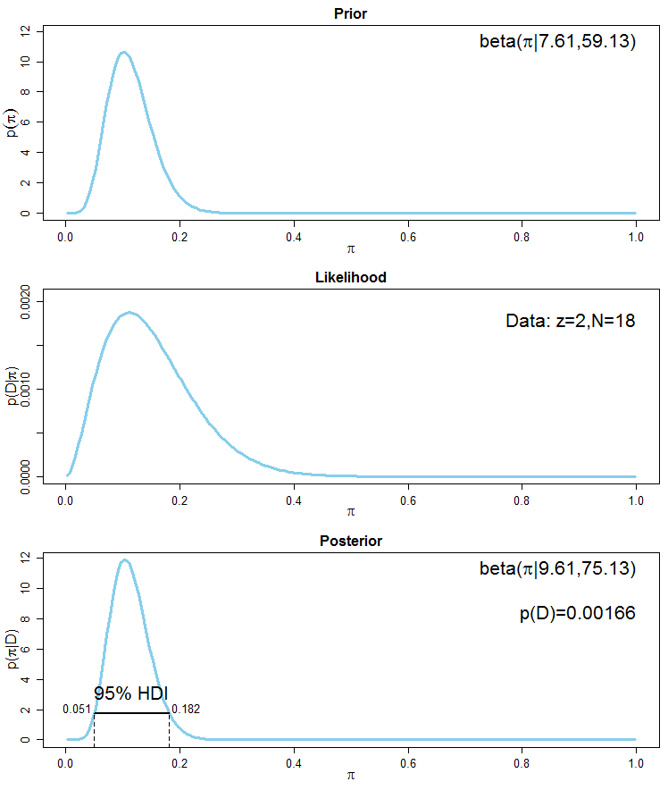
For standard distributions (e.g., normal, beta with certain parameters), you can sometimes solve for the HPD region in closed form. For a normal posterior , the HPD region is simply , which happens to equal the equal-tailed interval because the normal is symmetric.
From MCMC samples
Most practical Bayesian analyses use MCMC, so you'll compute HPD regions from posterior samples. Here's the standard approach for a unimodal, one-dimensional posterior:
- Sort the posterior samples in ascending order
- Consider all contiguous intervals that contain samples
- The shortest such interval is the HPD interval
This avoids density estimation entirely and works well with large sample sizes.
Kernel density estimation approach
For multimodal posteriors or when you need the actual density threshold:
-
Estimate the posterior density from MCMC samples using kernel density estimation (KDE)
-
Search for the threshold such that the region contains of the samples
-
Report all intervals where the estimated density exceeds
This method can capture disjoint HPD regions for multimodal posteriors, which the "shortest interval" method cannot.
High-dimensional challenges
In multiple dimensions, computing HPD regions becomes much harder. The "curse of dimensionality" makes density estimation unreliable, and visualizing the region is difficult beyond two dimensions. Common workarounds include computing marginal HPD intervals for each parameter separately or using dimension-reduction techniques.
Applications in Bayesian inference
Parameter estimation
HPD regions are the standard way to report uncertainty in Bayesian parameter estimates. A typical summary might read: "The posterior mode is 2.3, with a 95% HPD interval of [1.1, 3.8]." The asymmetry of the interval (wider on one side) immediately tells you the posterior is skewed.
Hypothesis testing
You can use HPD regions as a decision tool: if a hypothesized value (like for "no effect") falls outside the 95% HPD region, you have evidence against that hypothesis at the 5% level. This is analogous to checking whether a confidence interval contains zero, but with a direct probability interpretation.
Model comparison
Comparing HPD regions across competing models can reveal whether models agree on key parameters. If two models produce HPD regions with substantial overlap, they're telling a similar story about that parameter. Large discrepancies suggest the models differ meaningfully.
Interpretation and reporting
Graphical representation
The clearest way to show an HPD region is to shade the area under the posterior density curve between the HPD boundaries. For bivariate parameters, contour plots work well: the HPD region is the interior of the contour at height .
Confidence intervals vs. HPD regions
This distinction matters and comes up frequently on exams:
- A 95% HPD region means: "Given the data and prior, there is a 0.95 probability that lies in this region."
- A 95% confidence interval means: "If we repeated this experiment many times, 95% of the constructed intervals would contain the true ."
The HPD interpretation is a direct probability statement about the parameter. The confidence interval interpretation is about the procedure, not any single interval. Note that the HPD interpretation depends on the chosen prior.
Practical significance
A narrow HPD region indicates precise estimation; a wide one indicates substantial uncertainty. Beyond width, check whether the region includes or excludes values that matter for your research question. For example, if the 95% HPD for a treatment effect is [0.2, 1.8], the effect is credibly positive. If it's [-0.3, 1.5], you can't rule out zero effect.
Limitations and considerations
Multimodal distributions
When the posterior has multiple modes, the HPD region splits into separate pieces. Reporting "the 95% HPD region is [1.2, 2.1] ∪ [5.8, 7.3]" is correct but harder to interpret. In these cases, you should always include a plot of the full posterior so readers can see the multimodal structure.
Lack of transformation invariance
As noted above, HPD regions change when you reparameterize. If you compute an HPD region for and then transform to , the HPD region for won't simply be the log of the original boundaries. For problems where transformation invariance matters, equal-tailed intervals may be preferable.
Computational cost
For complex models with many parameters, accurately estimating HPD regions requires large MCMC samples and careful density estimation. The "shortest interval" method is fast but only works for unimodal, univariate cases. Multivariate or multimodal HPD regions demand more sophisticated (and slower) algorithms.
Comparison with other intervals
HPD vs. equal-tailed intervals
| Property | HPD Region | Equal-Tailed Interval |
|---|---|---|
| Width | Minimum for given probability | Can be wider for skewed posteriors |
| Symmetry | Matches posterior shape | Symmetric in probability (not width) |
| Contains mode | Always | Not necessarily |
| Transformation invariant | No | Yes |
| Handles multimodality | Yes (disjoint regions) | No |
| Ease of computation | Harder (needs density info) | Easier (just quantiles) |
HPD vs. frequentist confidence intervals
- HPD regions make direct probability statements; confidence intervals do not
- HPD regions incorporate prior information, which can yield narrower intervals with informative priors
- Confidence intervals don't require specifying a prior, which some view as an advantage
- With large samples and weak priors, the two often converge numerically
Software implementation
R packages
HDInterval: Thehdi()function computes HPD intervals directly from a vector of MCMC samplescoda: TheHPDinterval()function works with MCMC objects and is widely used with JAGS outputbayestestR: Provideshdi()along with other Bayesian summary tools
Python libraries
ArviZ: Theaz.hdi()function computes HPD intervals from posterior samples and integrates with PyMC and StanPyMC: Built-in summary functions include HPD intervals by defaultscipy.stats: Can be used for HPD computation on known parametric distributions
MCMC platforms
Stan and JAGS don't compute HPD regions internally, but their output (posterior samples) feeds directly into the R and Python tools listed above. The typical workflow is: run your sampler, extract samples, then compute HPD intervals in your analysis environment.
Advanced topics
HPD for mixture models
Mixture posteriors are inherently multimodal, so HPD regions will often be disjoint. Clustering algorithms (like Gaussian mixture models applied to the posterior samples) can help identify distinct modes before computing HPD regions around each one.
Time-varying HPD regions
In dynamic or state-space models, parameters change over time. You can compute HPD regions at each time step to visualize how uncertainty evolves. This is common in financial modeling and epidemiology, where tracking the width and location of HPD regions over time reveals periods of high vs. low uncertainty.
HPD in hierarchical models
Hierarchical models have parameters at multiple levels (e.g., group-level and population-level). You can compute HPD regions for each level separately. The population-level HPD region summarizes overall effects, while group-level HPD regions capture variation across groups. The high dimensionality of these models makes marginal HPD intervals (one parameter at a time) the most practical reporting choice.