Probability distributions are the backbone of Bayesian statistics, providing a mathematical framework for modeling uncertainty in data. They represent both prior beliefs and updated knowledge based on evidence, allowing us to quantify and reason about uncertainty in a systematic way.
Understanding different types of distributions, their properties, and how to work with them is crucial for effective Bayesian analysis. From discrete to continuous, univariate to multivariate, these distributions form the building blocks for complex statistical models and inference techniques.
Fundamentals of probability distributions
Probability distributions form the foundation of Bayesian statistics, providing a mathematical framework for modeling uncertainty and variability in data
In Bayesian analysis, probability distributions represent both prior beliefs and updated knowledge based on observed evidence
Concept of random variables
Top images from around the web for Concept of random variables
Discrete Random Variables | Boundless Statistics View original
Is this image relevant?
Frontiers | Indices of Effect Existence and Significance in the Bayesian Framework View original
Is this image relevant?
Bayesian Approaches | Mixed Models with R View original
Is this image relevant?
Discrete Random Variables | Boundless Statistics View original
Is this image relevant?
Frontiers | Indices of Effect Existence and Significance in the Bayesian Framework View original
Is this image relevant?
1 of 3
Random variables represent quantities with outcomes determined by chance or uncertainty
Discrete random variables take on countable values (coin flips, number of customers)
Continuous random variables can take any value within a range (height, temperature)
Probability distributions describe the likelihood of different outcomes for random variables
Probability mass vs density functions
Probability mass functions (PMFs) apply to discrete random variables
PMFs assign probabilities to specific values, summing to 1 across all possible outcomes
Probability density functions (PDFs) describe continuous random variables
PDFs represent relative likelihood, with area under the curve equaling 1
Interpret PDF values as probability densities, not direct probabilities
Cumulative distribution functions
Cumulative distribution functions (CDFs) apply to both discrete and continuous random variables
CDFs represent the probability of a random variable being less than or equal to a given value
For discrete variables, CDF is a step function
For continuous variables, CDF is a smooth, non-decreasing function
CDFs range from 0 to 1 and approach these limits as x approaches negative and positive infinity
Types of probability distributions
Probability distributions in Bayesian statistics model both prior beliefs and likelihood functions
Understanding different types of distributions helps in selecting appropriate models for various scenarios
Discrete vs continuous distributions
Discrete distributions model random variables with countable outcomes
Probability mass functions describe discrete distributions (binomial, Poisson)
Continuous distributions model random variables with uncountable outcomes
Probability density functions describe continuous distributions (normal, exponential)
Some distributions (gamma) can be discrete or continuous depending on
Univariate vs multivariate distributions
Univariate distributions describe a single random variable
Univariate distributions represented by single-variable functions ()
Multivariate distributions model multiple random variables simultaneously
describe relationships between variables
Covariance and correlation capture dependencies in multivariate distributions
Parametric vs nonparametric distributions
Parametric distributions defined by a fixed number of parameters
Common parametric distributions include normal (mean, variance) and exponential (rate)
Nonparametric distributions not constrained by fixed parameter set
Kernel density estimation creates flexible, data-driven distributions
Discrete distributions play a crucial role in Bayesian analysis for modeling countable outcomes
These distributions often serve as likelihood functions or priors in discrete data scenarios
Bernoulli distribution
Models binary outcomes with probability of success p and failure 1-p
: P(X=x)=px(1−p)1−x for x = 0 or 1
Mean: E[X]=p, Variance: Var(X)=p(1−p)
Used in Bayesian inference for binary classification problems
Binomial distribution
Extends Bernoulli to n independent trials with probability of success p
Probability mass function: P(X=k)=(kn)pk(1−p)n−k for k = 0, 1, ..., n
Mean: E[X]=np, Variance: Var(X)=np(1−p)
Applied in Bayesian analysis of proportions and count data
Poisson distribution
Models number of events in fixed time or space interval
Probability mass function: P(X=k)=k!λke−λ for k = 0, 1, 2, ...
Mean and variance both equal to rate parameter λ
Used in Bayesian modeling of rare events and time series data
Geometric distribution
Models number of trials until first success in Bernoulli trials
Probability mass function: P(X=k)=p(1−p)k−1 for k = 1, 2, 3, ...
Mean: E[X]=p1, Variance: Var(X)=p21−p
Applied in Bayesian survival analysis and reliability studies
Common continuous distributions
Continuous distributions are essential in Bayesian statistics for modeling real-valued data
These distributions often serve as priors or likelihood functions in continuous data scenarios
Uniform distribution
Models equal probability over a finite interval [a, b]
: f(x)=b−a1 for a ≤ x ≤ b
Mean: E[X]=2a+b, Variance: Var(X)=12(b−a)2
Often used as noninformative prior in Bayesian inference
Normal distribution
Bell-shaped distribution defined by mean μ and standard deviation σ
Probability density function: f(x)=σ2π1e−2σ2(x−μ)2
justifies its widespread use in Bayesian modeling
Conjugate prior for normal likelihood with known variance
Exponential distribution
Models time between events in Poisson process
Probability density function: f(x)=λe−λx for x ≥ 0
Mean: E[X]=λ1, Variance: Var(X)=λ21
Memoryless property: P(X>s+t∣X>s)=P(X>t)
Gamma distribution
Generalizes with shape α and rate β parameters
Probability density function: f(x)=Γ(α)βαxα−1e−βx for x > 0
Mean: E[X]=βα, Variance: Var(X)=β2α
Conjugate prior for Poisson and exponential likelihoods
Properties of distributions
Understanding distribution properties is crucial for effective Bayesian modeling and inference
These properties help in selecting appropriate priors and interpreting posterior distributions
Moments of distributions
Moments characterize the shape and behavior of probability distributions
First moment (mean) represents central tendency
Second moment relates to spread and variability
Higher moments describe , , and other shape characteristics
Moment-generating functions uniquely determine probability distributions
Expectation and variance
Expectation (E[X]) represents average or central value of a distribution
For discrete distributions: E[X]=∑xxP(X=x)
For continuous distributions: E[X]=∫−∞∞xf(x)dx
Variance (Var(X)) measures spread or dispersion around the mean
Calculated as Var(X)=E[(X−E[X])2]=E[X2]−(E[X])2
Skewness and kurtosis
Skewness measures asymmetry of probability distribution
Positive skew: right tail longer than left (income distributions)
Negative skew: left tail longer than right (exam scores)
Kurtosis quantifies tailedness or peakedness of distribution
Higher kurtosis indicates heavier tails and sharper peak
Normal distribution has kurtosis of 3 (mesokurtic)
Multivariate distributions
Multivariate distributions model relationships between multiple random variables
Essential for Bayesian analysis of complex systems and high-dimensional data
Joint probability distributions
Describe simultaneous behavior of multiple random variables
For discrete variables: P(X=x,Y=y) gives joint probability
For continuous variables: f(x,y) represents joint density function
Correlation and covariance capture linear relationships between variables
Copulas model complex dependencies in multivariate distributions
Marginal distributions
Obtained by integrating or summing joint distribution over other variables
For discrete variables: P(X=x)=∑yP(X=x,Y=y)
For continuous variables: fX(x)=∫−∞∞f(x,y)dy
discard information about relationships between variables
Used to analyze individual variables in multivariate settings
Conditional distributions
Describe distribution of one variable given known values of others
For discrete variables: P(X=x∣Y=y)=P(Y=y)P(X=x,Y=y)
For continuous variables: fX∣Y(x∣y)=fY(y)f(x,y)
Bayes' theorem relates conditional and marginal distributions
Crucial in Bayesian inference for updating beliefs given observed data
Transformations of random variables
Transformations allow manipulation of random variables to create new distributions
Understanding transformations is essential for deriving sampling distributions and posterior calculations
Linear transformations
Involve scaling and shifting random variables: Y = aX + b
Preserve shape of distribution but affect location and scale
Mean transforms as E[Y]=aE[X]+b
Variance transforms as Var(Y)=a2Var(X)
Useful for standardizing variables and creating z-scores
Non-linear transformations
Involve applying non-linear functions to random variables: Y = g(X)
Can significantly alter shape and properties of original distribution
Jacobian determinant required for transforming probability density functions
Moment-generating functions useful for deriving properties of transformed variables
Log-normal distribution arises from exponentiating normally distributed variable
Convolution of distributions
Describes sum of independent random variables
For discrete variables: P(X+Y=z)=∑xP(X=x)P(Y=z−x)
For continuous variables: fX+Y(z)=∫−∞∞fX(x)fY(z−x)dx
Convolution theorem simplifies calculations using Fourier transforms
Central Limit Theorem results from repeated convolutions
Bayesian perspective on distributions
Bayesian statistics treats parameters as random variables with associated distributions
This approach allows incorporation of prior knowledge and quantification of parameter uncertainty
Prior distributions
Represent initial beliefs about parameters before observing data
Can be informative (based on previous studies) or noninformative (uniform, Jeffreys prior)
simplify posterior calculations for certain likelihood functions
Hierarchical priors model parameter dependencies in complex models
Elicitation techniques help experts quantify prior beliefs
Likelihood functions
Describe probability of observed data given model parameters
Not a probability distribution over parameters, but function of parameters given fixed data
For independent observations: L(θ∣x)=∏i=1nf(xi∣θ)
Maximum likelihood estimation finds parameters maximizing likelihood
In Bayesian inference, likelihood combines with prior to form posterior
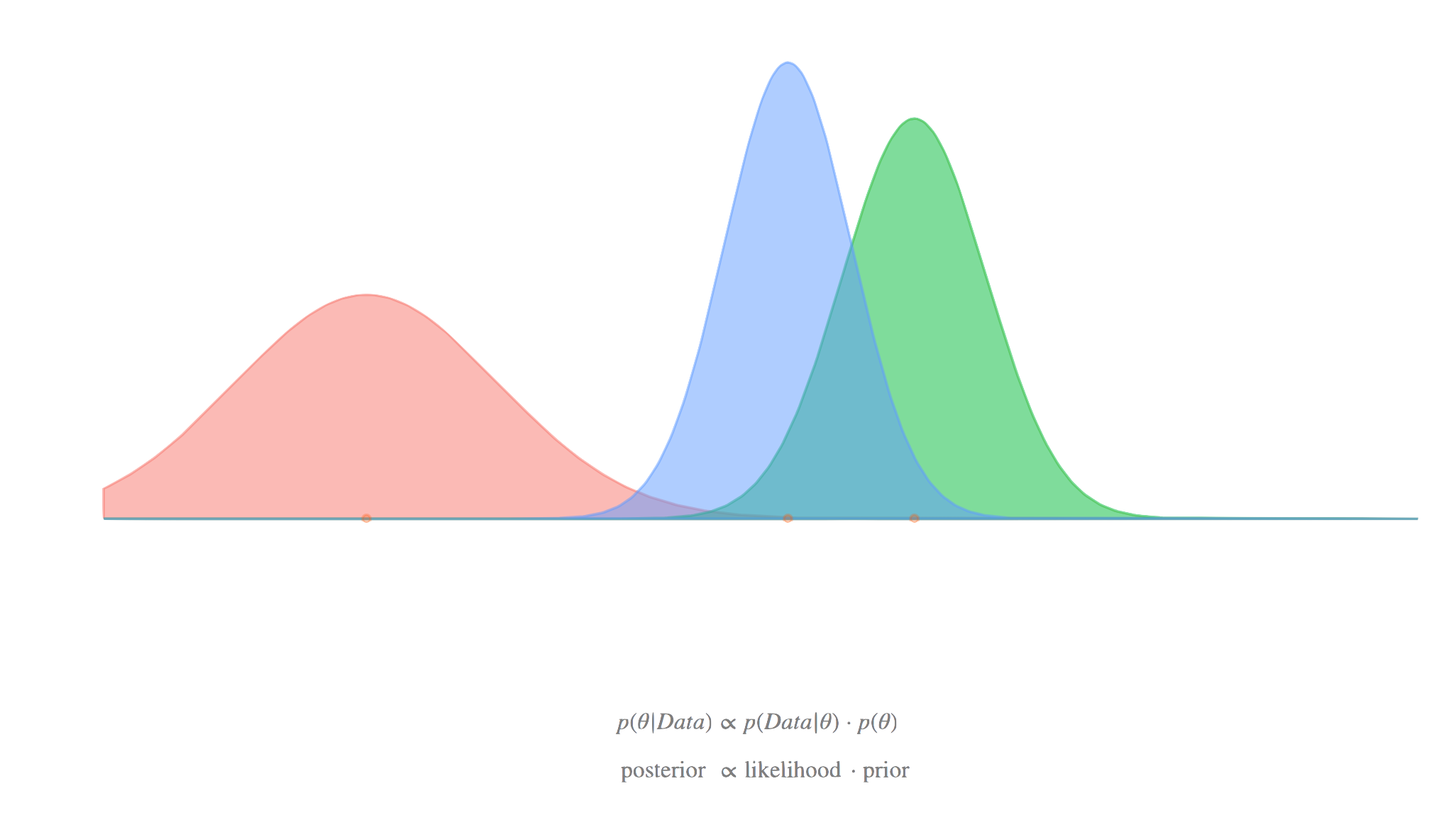
Posterior distributions
Represent updated beliefs about parameters after observing data
Calculated using Bayes' theorem: p(θ∣x)∝p(θ)L(θ∣x)
Often analytically intractable, requiring numerical approximation methods
Summarized using point estimates (MAP, posterior mean) and credible intervals
Posterior predictive distributions used for model checking and prediction
Sampling from distributions
Sampling techniques are crucial for Bayesian computation and Monte Carlo methods
These methods allow generation of random variables from complex distributions
Inverse transform sampling
Generates samples from any distribution with known (CDF)
Steps: generate U ~ Uniform(0,1), compute X = F^(-1)(U) where F is the CDF
Works well for distributions with analytically invertible CDFs (exponential, Cauchy)
Efficient for univariate distributions but challenging for multivariate cases
Forms basis for more advanced sampling methods (copula sampling)
Rejection sampling
Generates samples from target distribution using proposal distribution
Steps: sample from proposal, accept/reject based on ratio of target to proposal densities
Requires knowledge of upper bound on ratio of target to proposal densities
Efficiency depends on similarity between target and proposal distributions
Useful for sampling from distributions with complex shapes or truncated domains
Importance sampling
Estimates properties of target distribution using samples from proposal distribution
Assigns weights to samples based on ratio of target to proposal densities
Effective for estimating expectations and normalizing constants
Self-normalized importance sampling corrects for unknown normalizing constants
Forms basis for particle filtering methods in sequential Monte Carlo
Applications in Bayesian inference
Probability distributions play central role in Bayesian modeling and inference
Understanding distribution properties and relationships is crucial for effective Bayesian analysis
Conjugate priors
Prior distributions that yield posterior distributions in same family as prior
Simplify posterior calculations and enable closed-form solutions
Beta prior conjugate to binomial likelihood for inference on proportions
Normal-Inverse-Gamma prior conjugate to normal likelihood for unknown mean and variance
Trade-off between computational convenience and flexibility in prior specification
Hierarchical models
Model parameters as drawn from higher-level distributions
Allow sharing of information across groups or subpopulations
Hyperparameters control overall behavior of lower-level parameters
Often implemented using normal or Student's t distributions for shrinkage
Facilitate partial pooling between complete pooling and no pooling extremes
Mixture models
Represent complex distributions as weighted sum of simpler component distributions
Gaussian use weighted sum of normal distributions
Dirichlet process mixtures allow infinite number of components
Useful for clustering, density estimation, and modeling heterogeneous populations
Expectation-Maximization (EM) algorithm commonly used for fitting mixture models
Key Terms to Review (31)
Binomial Distribution: The binomial distribution is a probability distribution that models the number of successes in a fixed number of independent Bernoulli trials, each with the same probability of success. This distribution is crucial for understanding the behavior of random variables that have two possible outcomes, like flipping a coin or passing a test, and plays a key role in probability distributions and maximum likelihood estimation.
Bootstrap sampling: Bootstrap sampling is a resampling technique that involves repeatedly drawing samples, with replacement, from a single dataset to estimate the sampling distribution of a statistic. This method is particularly useful for estimating the confidence intervals and biases of estimators when the underlying distribution is unknown or when the sample size is small. By creating multiple simulated samples, bootstrap sampling helps in understanding the variability of a statistic and makes it possible to perform inference without relying on traditional parametric assumptions.
Central Limit Theorem: The Central Limit Theorem (CLT) states that, regardless of the original distribution of a dataset, the sampling distribution of the sample mean will tend to be normally distributed as the sample size becomes larger. This theorem is foundational because it allows statisticians to make inferences about population parameters using sample statistics, even when the underlying distribution is not normal. The CLT connects closely with probability distributions and plays a crucial role in methods like Monte Carlo integration by enabling the approximation of complex distributions.
Conditional Distributions: Conditional distributions refer to the probability distribution of a subset of variables given the values of other variables. This concept allows us to understand how the probabilities of certain events or outcomes change when we have information about other related events. Conditional distributions are essential for analyzing joint distributions, and they play a vital role in the realm of Bayesian statistics by helping to update our beliefs based on new evidence.
Conjugate Priors: Conjugate priors are a type of prior distribution that, when combined with a certain likelihood function, results in a posterior distribution that belongs to the same family as the prior. This property simplifies the process of updating beliefs with new evidence, making calculations more straightforward and efficient. The use of conjugate priors is particularly beneficial when dealing with Bayesian inference, as it leads to easier derivation of posterior distributions and facilitates model comparison methods.
Continuous random variable: A continuous random variable is a type of variable that can take on an infinite number of values within a given range. Unlike discrete random variables, which have specific, separate values, continuous random variables can represent measurements and can take any value, including fractions and decimals. This property is crucial for modeling real-world phenomena, especially when we deal with probabilities and statistical analysis.
Convolution of Distributions: The convolution of distributions is a mathematical operation that combines two probability distributions to produce a new distribution. This process reflects the distribution of the sum of two independent random variables, where each random variable is associated with one of the original distributions. The convolution effectively allows for the analysis of the combined behavior of these variables, which is particularly useful in various statistical applications.
Cumulative Distribution Function: A cumulative distribution function (CDF) is a statistical function that describes the probability that a random variable takes on a value less than or equal to a specific value. The CDF provides a complete description of the probability distribution of a random variable, allowing us to understand how probabilities accumulate across different values. It plays a crucial role in understanding both discrete and continuous random variables and their associated probability distributions.
Degrees of Freedom: Degrees of freedom refer to the number of independent values or quantities that can vary in an analysis without violating any constraints. In the context of probability distributions, this concept helps determine the number of parameters that can be freely estimated from the available data, influencing the shape and behavior of different statistical models. Understanding degrees of freedom is crucial for making inferences about populations from samples, as it directly impacts the calculations for various statistical tests and models.
Discrete random variable: A discrete random variable is a type of variable that can take on a countable number of distinct values, often representing outcomes of a random process. These variables are essential in statistical analysis as they allow for the modeling and understanding of phenomena that involve specific, separate outcomes. They help in defining probability distributions, calculating expectations, and assessing variance, thereby providing a structured way to analyze uncertainty and randomness in real-world scenarios.
Exponential Distribution: The exponential distribution is a probability distribution that describes the time between events in a Poisson process, which is a process that models random events occurring independently at a constant average rate. It is commonly used to model the time until an event occurs, such as the time until a radioactive particle decays or the time between arrivals at a service point. This distribution is characterized by its memoryless property, meaning that the future probability of an event does not depend on how much time has already passed.
Gamma Distribution: The gamma distribution is a continuous probability distribution that is used to model the time until an event occurs, especially when the events happen independently and continuously over time. It is defined by two parameters: the shape parameter (k) and the scale parameter (θ), which influence its shape and variance. This distribution plays an essential role in Bayesian statistics, particularly in modeling waiting times and in various applications like queuing theory and reliability analysis.
Geometric Distribution: The geometric distribution is a probability distribution that models the number of trials needed to achieve the first success in a sequence of independent Bernoulli trials. It helps understand scenarios where events occur randomly and independently, particularly focusing on the count of failures before the first success. This distribution is important for analyzing waiting times and can provide insights into the likelihood of various outcomes based on a given probability of success.
Hierarchical models: Hierarchical models are statistical models that are structured in layers, allowing for the incorporation of multiple levels of variability and dependencies. They enable the analysis of data that is organized at different levels, such as individuals nested within groups, making them particularly useful in capturing relationships and variability across those levels. This structure allows for more complex modeling of real-world situations, connecting to various aspects like probability distributions, model comparison, and sampling techniques.
Joint Probability Distributions: A joint probability distribution is a statistical representation that shows the probability of two or more random variables occurring simultaneously. This distribution captures the relationships between the variables, providing insight into how one variable might affect another, which is essential for understanding dependencies in data.
Kurtosis: Kurtosis is a statistical measure that describes the shape of a probability distribution's tails in relation to its overall shape. Specifically, it indicates how heavily the tails of the distribution differ from those of a normal distribution, providing insight into the presence of outliers. A higher kurtosis value suggests a distribution with heavier tails and more extreme outliers, while lower values indicate lighter tails and fewer outliers.
Law of Large Numbers: The law of large numbers is a statistical theorem that states as the size of a sample increases, the sample mean will get closer to the expected value (or population mean). This principle is foundational in probability and helps to justify the use of probability distributions in estimating outcomes, ensuring that the more observations we collect, the more accurate our estimations become.
Linear Transformations: Linear transformations are mathematical functions that map vectors from one vector space to another while preserving the operations of vector addition and scalar multiplication. They play a crucial role in understanding how probability distributions behave under changes such as scaling or shifting, which can be essential when modeling data in Bayesian statistics.
Marginal distributions: Marginal distributions refer to the probability distribution of a subset of a collection of random variables. They provide insights into the behavior of individual variables while accounting for the overall joint distribution of the variables involved. Understanding marginal distributions is crucial because they help simplify complex multivariate scenarios by allowing analysis of one variable at a time, without the influence of others.
Mixture Models: Mixture models are statistical models that represent a distribution as a combination of multiple component distributions, each corresponding to a different underlying process or group within the data. They are particularly useful for modeling complex datasets that exhibit heterogeneity, where individual observations may arise from different subpopulations or categories. By capturing this structure, mixture models help in identifying distinct groups and understanding the variability within the data, making them relevant in probability distributions and multiple hypothesis testing contexts.
Moments of Distributions: Moments of distributions are quantitative measures that capture various characteristics of a probability distribution, such as its central tendency and variability. The most commonly used moments include the mean, variance, skewness, and kurtosis, which provide insights into the shape and behavior of the distribution. Understanding these moments is essential for analyzing and interpreting statistical data effectively.
Non-linear transformations: Non-linear transformations refer to changes applied to data or functions that do not follow a straight line or proportionality, leading to altered probability distributions. These transformations can affect the shape, location, and scale of distributions, and often require special consideration in statistical modeling. Understanding how these transformations work is crucial for interpreting results and making predictions in Bayesian Statistics.
Normal Distribution: Normal distribution is a probability distribution that is symmetric about the mean, showing that data near the mean are more frequent in occurrence than data far from the mean. This bell-shaped curve is fundamental in statistics because it describes how variables are distributed and plays a crucial role in many statistical methods and theories.
Parameters: Parameters are numerical values that summarize characteristics of a probability distribution, such as location, scale, or shape. They play a crucial role in defining the specific behavior and properties of a distribution, allowing statisticians to make inferences and predictions about data based on these values.
Poisson Distribution: The Poisson distribution is a probability distribution that expresses the probability of a given number of events occurring in a fixed interval of time or space, given that these events occur with a known constant mean rate and independently of the time since the last event. It is commonly used in scenarios where events happen randomly and independently, making it a key concept in understanding random variables and their associated probability distributions.
Probability Density Function: A probability density function (PDF) is a statistical function that describes the likelihood of a continuous random variable taking on a specific value. The PDF is essential for understanding how probabilities are distributed over different values of the variable, allowing for calculations of probabilities over intervals rather than specific points. The area under the curve of a PDF across a certain range gives the probability that the random variable falls within that range.
Probability Mass Function: A probability mass function (PMF) is a function that gives the probability that a discrete random variable is equal to a specific value. It describes the distribution of probabilities across the different possible outcomes of a discrete random variable, ensuring that the total probability across all outcomes sums up to one. The PMF helps in understanding how probabilities are distributed among discrete events, providing a foundational tool for statistical analysis.
Sampling Distribution: A sampling distribution is the probability distribution of a statistic obtained through a large number of samples drawn from a specific population. This concept is key to understanding how sample statistics behave and helps in making inferences about the population parameters. It essentially describes the likelihood of different outcomes when you repeatedly take samples from a population and compute a statistic, such as the mean or variance.
Skewness: Skewness is a statistical measure that describes the asymmetry of a probability distribution. It indicates whether the data points in a distribution are concentrated on one side of the mean or the other, which can provide insights into the underlying characteristics of the dataset. Understanding skewness helps in assessing how normal a distribution is, as well as influencing decisions about appropriate statistical methods to apply.
Transformations of Random Variables: Transformations of random variables refer to the process of applying a mathematical function to a random variable, which results in a new random variable. This concept is crucial as it allows statisticians to understand how changes in data or model specifications affect probability distributions, thereby facilitating the analysis and interpretation of random phenomena.
Uniform Distribution: A uniform distribution is a type of probability distribution where all outcomes are equally likely to occur. This concept plays a crucial role in understanding random variables, probability distributions, expectation and variance, and even Monte Carlo integration, as it provides a foundational model for scenarios where every event has the same chance of happening, making it simple to calculate probabilities and expectations.