7.1 Ridge Regression: L2 Regularization

Ridge regression adds a penalty term to linear regression, shrinking coefficients towards zero. This L2 regularization technique helps prevent overfitting and handles multicollinearity, striking a balance between model complexity and performance.

The regularization parameter λ controls the strength of shrinkage. As λ increases, coefficients are pulled closer to zero. Cross-validation helps find the optimal λ, balancing bias and variance for better generalization.

Ridge Regression Fundamentals

Overview and Key Concepts

• Ridge regression extends linear regression by adding a penalty term to the ordinary least squares (OLS) objective function
• L2 regularization refers to the specific type of penalty used in ridge regression, which is the sum of squared coefficients multiplied by the regularization parameter
• The penalty term in ridge regression is $\lambda \sum_{j=1}^{p} \beta_j^2$, where $\lambda$ is the regularization parameter and $\beta_j$ are the regression coefficients
  • This penalty term is added to the OLS objective function, resulting in the ridge regression objective: $\sum_{i=1}^{n} (y_i - \beta_0 - \sum_{j=1}^{p} \beta_j x_{ij})^2 + \lambda \sum_{j=1}^{p} \beta_j^2$
• The regularization parameter $\lambda$ controls the strength of the penalty
  • When $\lambda = 0$, ridge regression reduces to OLS
  • As $\lambda \to \infty$, the coefficients are shrunk towards zero
• Shrinkage refers to the effect of the penalty term, which shrinks the regression coefficients towards zero compared to OLS
  • This can help prevent overfitting and improve the model's generalization performance

Geometric Interpretation

• Ridge regression can be interpreted as a constrained optimization problem
  • The objective is to minimize the RSS (residual sum of squares) subject to a constraint on the L2 norm of the coefficients: $\sum_{j=1}^{p} \beta_j^2 \leq t$, where $t$ is a tuning parameter related to $\lambda$
• Geometrically, this constraint corresponds to a circular region in the parameter space
  • The ridge regression solution is the point where the RSS contour lines first touch this circular constraint region
• As the constraint becomes tighter (smaller $t$, larger $\lambda$), the solution is pulled further towards the origin, resulting in greater shrinkage of the coefficients

Benefits and Tradeoffs

Bias-Variance Tradeoff

• Ridge regression can improve a model's performance by reducing its variance at the cost of slightly increasing its bias
  • The penalty term constrains the coefficients, limiting the model's flexibility and thus reducing variance
  • However, this constraint also introduces some bias, as the coefficients are shrunk towards zero and may not match the true underlying values
• The bias-variance tradeoff is controlled by the regularization parameter $\lambda$
  • Larger $\lambda$ values result in greater shrinkage, lower variance, and higher bias
  • Smaller $\lambda$ values result in less shrinkage, higher variance, and lower bias
• The optimal $\lambda$ value can be selected using techniques like cross-validation to balance bias and variance and minimize the model's expected test error

Handling Multicollinearity

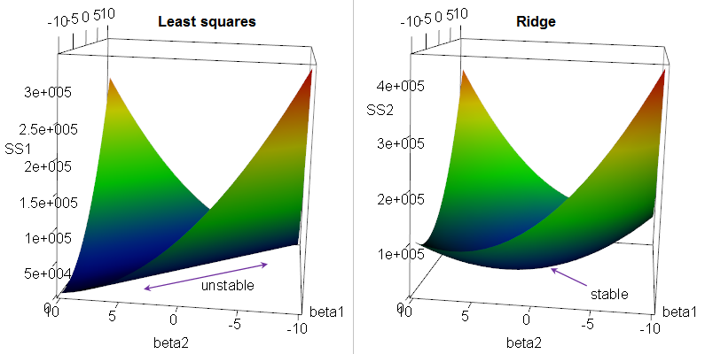
• Multicollinearity occurs when predictor variables in a regression model are highly correlated with each other
  • This can lead to unstable and unreliable coefficient estimates in OLS
• Ridge regression can effectively handle multicollinearity by shrinking the coefficients of correlated predictors towards each other
  • This results in a more stable and interpretable model, as the impact of multicollinearity on the coefficient estimates is reduced
• When predictors are highly correlated, ridge regression tends to assign similar coefficients to them, reflecting their shared contribution to the response variable

Model Selection via Cross-Validation

• Cross-validation is commonly used to select the optimal value of the regularization parameter $\lambda$ in ridge regression
• The procedure involves:
  1. Splitting the data into $k$ folds
  2. For each $\lambda$ value in a predefined grid:
     • Train ridge regression models on $k-1$ folds and evaluate their performance on the held-out fold
     • Repeat this process $k$ times, using each fold as the validation set once
     • Compute the average performance across the $k$ folds
  3. Select the $\lambda$ value that yields the best average performance
• This process helps identify the $\lambda$ value that strikes the best balance between bias and variance, optimizing the model's expected performance on new, unseen data

Solving Ridge Regression

Closed-Form Solution

• Ridge regression has a closed-form solution, which can be derived analytically by solving the normal equations with the addition of the penalty term
• The closed-form solution for ridge regression is given by: $\hat{\beta}^{ridge} = (\mathbf{X}^T\mathbf{X} + \lambda \mathbf{I})^{-1} \mathbf{X}^T \mathbf{y}$ where:
  • $\mathbf{X}$ is the $n \times p$ matrix of predictor variables
  • $\mathbf{y}$ is the $n \times 1$ vector of response values
  • $\lambda$ is the regularization parameter
  • $\mathbf{I}$ is the $p \times p$ identity matrix
• Compared to the OLS solution $\hat{\beta}^{OLS} = (\mathbf{X}^T\mathbf{X})^{-1} \mathbf{X}^T \mathbf{y}$, ridge regression adds the term $\lambda \mathbf{I}$ to the matrix $\mathbf{X}^T\mathbf{X}$ before inversion
  • This addition makes the matrix $\mathbf{X}^T\mathbf{X} + \lambda \mathbf{I}$ invertible even when $\mathbf{X}^T\mathbf{X}$ is not (e.g., in the presence of perfect multicollinearity)
  • The closed-form solution for ridge regression is computationally efficient and numerically stable, even when dealing with high-dimensional data or correlated predictors