takes linear regression up a notch by adding curved terms. This lets us model wiggly relationships between variables, like how your income might peak in middle age. It's super flexible but can go overboard if we're not careful.

To avoid fitting every little blip in our data, we can use tricks like or . We can also try , which are like connecting the dots with smooth curves. These tools help us find the sweet spot between too simple and too complex.

Polynomial Regression Models

Polynomial Terms and Model Complexity

Top images from around the web for Polynomial Terms and Model Complexity
  • Polynomial regression models extend linear regression by adding polynomial terms of the predictor variables
    • Allows modeling non-linear relationships between predictors and the response variable
    • Polynomial terms are created by raising each predictor to a power (e.g., x2x^2, x3x^3)
  • increases as higher degree polynomial terms are added
    • Higher degree polynomials can fit more complex, non-linear patterns in the data
    • Increases the flexibility of the model to capture intricate relationships
    • Must be balanced against the risk of

Quadratic and Cubic Regression

  • includes polynomial terms up to degree 2 for each predictor
    • Adds squared terms like x12x_1^2, x22x_2^2 to the model
    • Can model relationships where the response increases then decreases (or vice versa) as the predictor changes
    • Example: Modeling the relationship between age and income, where income may peak at middle age
  • includes polynomial terms up to degree 3
    • Adds cubed terms like x13x_1^3, x23x_2^3 in addition to squared terms
    • Can capture more complex non-linear patterns with multiple bends or inflection points
    • Provides greater flexibility than quadratic regression but with increased complexity
    • Example: Modeling the relationship between temperature and crop yield, where yield may have multiple peaks and valleys at different temperature ranges

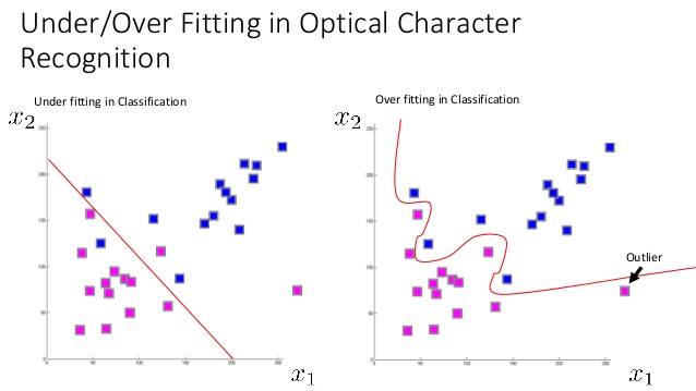
Overfitting and Complexity

Overfitting in Polynomial Regression

  • Overfitting occurs when a model is too complex and fits the noise in the training data rather than the underlying pattern
    • Model performs well on training data but poorly on new, unseen data
    • High degree polynomial terms can lead to overfitting by capturing random fluctuations
  • Overfitting can be mitigated by:
    • Regularization techniques (e.g., , ) that penalize large coefficients
    • Cross-validation to assess model performance on held-out data and select appropriate complexity
    • Limiting the terms based on domain knowledge or data exploration

Basis Functions and Splines

  • are a set of functions used to represent the predictor variables in a regression model
    • Polynomial terms (e.g., xx, x2x^2, x3x^3) are a type of basis function
    • Other basis functions include trigonometric functions, wavelets, and splines
  • Splines are piecewise polynomial functions used to model complex non-linear relationships
    • Divide the range of a predictor into segments and fit separate low-degree polynomials in each segment
    • Ensure continuity and smoothness at the segment boundaries (knots)
    • Examples include cubic splines, B-splines, and natural splines
  • Splines provide a flexible way to model non-linear relationships while controlling complexity
    • Knot locations and the degree of polynomials can be chosen to balance fit and smoothness
    • Regularization can be applied to spline coefficients to prevent overfitting

Key Terms to Review (27)

Basis functions: Basis functions are a set of functions used to represent data in a transformed space, allowing for flexible modeling of relationships between variables. They form the building blocks of more complex functions, enabling the approximation of non-linear patterns in data. These functions are particularly useful in smoothing techniques and flexible modeling approaches, facilitating the exploration of underlying trends without being overly rigid.
Coefficient: A coefficient is a numerical value that represents the strength and direction of the relationship between a predictor variable and the response variable in regression analysis. In polynomial regression, coefficients are crucial as they determine the shape of the polynomial curve, allowing for the modeling of non-linear relationships by adjusting how each term contributes to the prediction. Each coefficient corresponds to a specific power of the independent variable, influencing how changes in that variable affect the output.
Condition Number: The condition number is a measure of how sensitive a function's output is to changes in its input. It plays a crucial role in understanding the stability of polynomial regression models, especially when dealing with non-linear relationships. A high condition number indicates that small changes in the input can lead to large variations in the output, which can significantly affect the model's predictions and overall performance.
Cross-validation: Cross-validation is a statistical technique used to assess the performance of a predictive model by dividing the dataset into subsets, training the model on some of these subsets while validating it on the remaining ones. This process helps to ensure that the model generalizes well to unseen data and reduces the risk of overfitting by providing a more reliable estimate of its predictive accuracy.
Cubic Regression: Cubic regression is a type of polynomial regression that uses a cubic function to model the relationship between a dependent variable and one or more independent variables. It allows for more flexibility than linear or quadratic models, enabling the capture of complex, non-linear relationships in the data, often characterized by its ability to create an S-shaped curve. This can be particularly useful when the relationship exhibits curvature, providing a better fit for datasets that do not follow a straight line or simple parabolic form.
Curve fitting: Curve fitting is the process of constructing a curve or mathematical function that best approximates the relationship between a set of data points. This technique is essential for modeling complex relationships in data, helping to identify trends and make predictions based on the available information. Various methods exist for curve fitting, including polynomial regression and spline fitting, which allow for flexibility in adapting to non-linear relationships found in real-world data.
Degree of polynomial: The degree of a polynomial is the highest power of the variable in the polynomial expression. It indicates the polynomial's complexity and plays a crucial role in determining its shape, behavior, and the nature of its roots. Understanding the degree helps in polynomial regression as it affects how well the model can fit non-linear relationships between variables.
Gradient descent: Gradient descent is an optimization algorithm used to minimize the loss function in various machine learning models by iteratively updating the model parameters in the direction of the steepest descent of the loss function. This method is crucial for training models, as it helps find the optimal parameters that minimize prediction errors and improves model performance. By leveraging gradients, gradient descent connects closely with regularization techniques, neural network training, computational efficiency, and the handling of complex non-linear relationships.
Lasso: Lasso, short for Least Absolute Shrinkage and Selection Operator, is a regression analysis method that performs both variable selection and regularization to enhance the prediction accuracy and interpretability of statistical models. It adds a penalty equal to the absolute value of the magnitude of coefficients, which encourages simpler models by forcing some coefficients to be exactly zero. This is particularly useful when dealing with high-dimensional data, making it easier to identify relevant predictors.
Least Squares Estimation: Least squares estimation is a mathematical approach used to determine the best-fitting line or model for a set of data by minimizing the sum of the squares of the differences between observed and predicted values. This technique is fundamental in regression analysis, ensuring that predictions are as accurate as possible while allowing for easy interpretation of relationships between variables. It serves as a cornerstone for various regression techniques, making it essential for both linear and non-linear modeling applications.
Linearity Assumption: The linearity assumption is the premise that the relationship between the independent and dependent variables in a model can be accurately described by a straight line. This assumption is critical because it influences how we interpret the results of regression analyses and affects the accuracy of predictions. When this assumption holds true, it ensures that the model captures the relationship effectively; however, violating this assumption can lead to misleading conclusions and necessitate adjustments such as polynomial regression or transformations.
Logarithmic transformation: A logarithmic transformation is a mathematical technique used to compress the range of data values by applying a logarithm function, often the natural logarithm, to the data. This transformation is particularly useful when dealing with data that exhibits exponential growth or positive skewness, allowing for a more linear relationship in regression models and enhancing the interpretability of results.
Mean Squared Error: Mean Squared Error (MSE) is a measure used to evaluate the accuracy of a predictive model by calculating the average of the squares of the errors, which are the differences between predicted and actual values. It plays a crucial role in supervised learning by quantifying how well models are performing, affecting decisions in model selection, bias-variance tradeoff, regularization techniques, and more.
Model complexity: Model complexity refers to the capacity of a statistical model to fit a wide variety of data patterns. It is influenced by the number of parameters in the model and can affect how well the model generalizes to unseen data. Understanding model complexity is essential for balancing the need for a flexible model that can capture relationships in the data while avoiding overfitting.
Non-linear regression: Non-linear regression is a form of regression analysis in which the relationship between the independent variable(s) and the dependent variable is modeled as a non-linear function. This technique is particularly useful when data shows complex patterns that cannot be accurately captured with a straight line, allowing for better fitting of curves or other non-linear shapes to the data points.
Normality Assumption: The normality assumption is the premise that the residuals (the differences between observed and predicted values) of a regression model are normally distributed. This assumption is critical because many statistical tests and methods, including hypothesis testing and confidence intervals, rely on this property to ensure validity. When analyzing models, confirming the normality of residuals helps in validating model performance and drawing reliable conclusions.
Overfitting: Overfitting occurs when a statistical model or machine learning algorithm captures noise or random fluctuations in the training data instead of the underlying patterns, leading to poor generalization to new, unseen data. This results in a model that performs exceptionally well on training data but fails to predict accurately on validation or test sets.
Polynomial regression: Polynomial regression is a type of regression analysis that models the relationship between a dependent variable and one or more independent variables as an nth degree polynomial. This approach is particularly useful for capturing non-linear relationships between variables, allowing for a more flexible fitting of the data compared to simple linear regression, which only considers straight-line relationships.
Power Transformation: Power transformation is a technique used in statistical modeling to stabilize variance and make data more normally distributed by applying a power function to the variables. This process is essential when dealing with non-linear relationships in data, as it helps improve the accuracy of polynomial regression models and better captures complex patterns in the dataset.
Quadratic regression: Quadratic regression is a type of polynomial regression where the relationship between the independent variable and the dependent variable is modeled as a second-degree polynomial. This approach is particularly useful for capturing non-linear relationships in data, allowing for a parabolic curve that can better fit certain datasets compared to linear regression. By fitting a quadratic equation of the form $$y = ax^2 + bx + c$$ to the data, it can account for curvature in the data that simple linear models cannot capture.
R-squared: R-squared, also known as the coefficient of determination, is a statistical measure that represents the proportion of the variance for a dependent variable that can be explained by one or more independent variables in a regression model. It helps evaluate the effectiveness of a model and is crucial for understanding model diagnostics, bias-variance tradeoff, and regression metrics.
Regularization: Regularization is a technique used in statistical learning and machine learning to prevent overfitting by adding a penalty term to the loss function, which discourages overly complex models. This method helps in balancing model complexity and performance by penalizing large coefficients, ultimately leading to better generalization on unseen data.
Ridge regression: Ridge regression is a type of linear regression that incorporates L2 regularization to prevent overfitting by adding a penalty equal to the square of the magnitude of coefficients. This approach helps manage multicollinearity in multiple linear regression models and improves prediction accuracy, especially when dealing with high-dimensional data. Ridge regression is closely related to other regularization techniques and model evaluation criteria, making it a key concept in statistical modeling and machine learning.
Splines: Splines are piecewise polynomial functions that are used to create smooth curves through a set of data points. They are particularly useful in regression analysis for modeling non-linear relationships, allowing for flexibility in fitting data without overfitting as compared to high-degree polynomial regression.
Trend Analysis: Trend analysis is a statistical technique used to identify patterns or trends in data over time, which helps in understanding underlying behaviors and predicting future outcomes. By examining historical data, it allows for the assessment of changes, enabling better decision-making and forecasting in various contexts, including relationships between variables and potential non-linear patterns. This method is fundamental in numerous analytical techniques that aim to capture the essence of data behavior across different intervals.
Underfitting: Underfitting occurs when a statistical model is too simple to capture the underlying structure of the data, resulting in poor predictive performance. This typically happens when the model has high bias and fails to account for the complexity of the data, leading to systematic errors in both training and test datasets.
Variance Inflation Factor: Variance inflation factor (VIF) is a measure used to detect multicollinearity in multiple linear regression models. It quantifies how much the variance of an estimated regression coefficient increases when your predictors are correlated. A high VIF indicates that the predictor may be providing redundant information about the response variable, which can lead to unstable estimates and difficulties in determining the significance of predictors.
© 2024 Fiveable Inc. All rights reserved.
AP® and SAT® are trademarks registered by the College Board, which is not affiliated with, and does not endorse this website.