Addressing Non-normality of Residuals
Detecting Non-normality
Residuals in linear regression need to follow a normal distribution for your inference (confidence intervals, hypothesis tests) to be valid. When this assumption breaks down, you get biased standard errors, unreliable confidence intervals, and p-values you can't trust.
You can spot non-normality two ways:
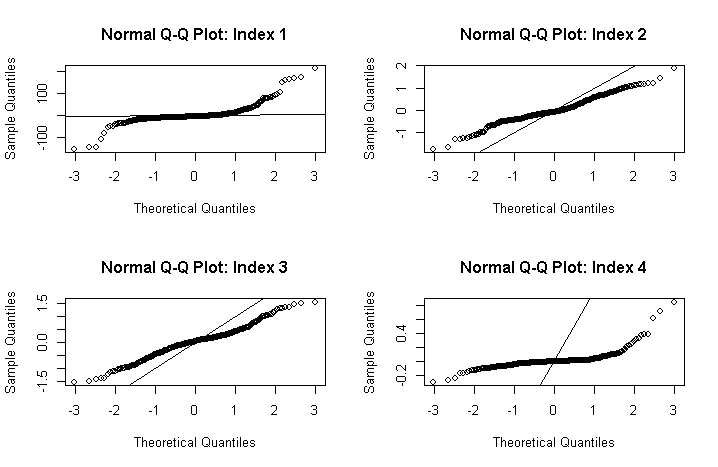
- Visual inspection: Look at a histogram of residuals or a Q-Q plot. In the Q-Q plot, points should fall roughly along the diagonal line. Systematic departures (S-curves, bowing) signal trouble.
- Formal tests: The Shapiro-Wilk test and Anderson-Darling test both test the null hypothesis that residuals are normally distributed. A small p-value means you reject normality.
Non-normality typically shows up as skewness, heavy tails, or influential outliers in the residual distribution.
Applying Transformations
The most common fix for non-normal residuals is transforming the response variable. Three standard options:
- Logarithmic transformation works well for right-skewed residuals, which are common with variables like income or prices that are bounded below by zero and have a long right tail.
- Square root transformation is a milder correction, appropriate for moderately right-skewed residuals. Count data often benefits from this.
- Box-Cox transformation is the most flexible option. It estimates an optimal power parameter from the data itself, so you don't have to guess which transformation fits best. When , it reduces to the log transform; when , it approximates the square root.
After transforming and refitting the model, reassess the residuals. If normality still doesn't hold, you may need to try a different transformation or move to non-parametric methods.
Interpreting transformed models: Coefficients and predictions live on the transformed scale. You'll often need to back-transform for meaningful interpretation. For example, in a log-transformed model, a coefficient of 0.5 means a one-unit increase in the predictor multiplies the response by on the original scale.
Handling Heteroscedasticity
Identifying Heteroscedasticity
Heteroscedasticity means the variance of the residuals changes across the range of fitted values, violating the constant-variance (homoscedasticity) assumption. A classic example: residuals that fan out as predicted values increase, forming a "megaphone" shape.
Detection approaches:
- Residuals vs. fitted values plot: Look for any systematic pattern in the spread of residuals. Constant spread means homoscedasticity; a funnel or wedge shape means heteroscedasticity.
- Breusch-Pagan test: Regresses squared residuals on the predictors. A significant result indicates the variance depends on the predictors.
- White's test: A more general version that also checks for nonlinear forms of heteroscedasticity.
When heteroscedasticity is present but ignored, your coefficient estimates are still unbiased, but they're no longer efficient. More critically, your standard errors become biased, which invalidates hypothesis tests and confidence intervals.
Implementing Weighted Least Squares (WLS)
Weighted least squares corrects heteroscedasticity by giving each observation a weight inversely related to its variance. The logic: observations with large variance are less informative, so they should count less.
How WLS works, step by step:
-
Fit the ordinary least squares (OLS) model and examine the residuals for heteroscedasticity.
-
Estimate the variance function, which models how residual variance relates to the predictors. Common choices include:
- Inverse variance weights:
- Weights based on squared residuals:
- A parametric function of predictors:
-
Multiply both sides of the regression equation by , transforming the model so that the weighted residuals have constant variance.
-
Estimate the transformed model using ordinary least squares.
-
Re-check the weighted residuals for any remaining heteroscedasticity.
WLS gives you more efficient, unbiased estimates compared to OLS when heteroscedasticity is present. The catch is that you need to specify the variance function correctly. If you get the variance function wrong, your estimates can actually become biased, so this step deserves careful attention.
Mitigating Multicollinearity
Understanding Multicollinearity
Multicollinearity occurs when predictor variables in a multiple regression model are highly correlated with each other. This doesn't bias your coefficient estimates, but it inflates their standard errors, making individual coefficients unstable and hard to interpret. Small changes in the data can cause large swings in the estimated coefficients.
Detection tools:
- Correlation matrix: Pairwise correlations above roughly 0.8 between predictors are a warning sign, though multicollinearity can exist even without any single high pairwise correlation.
- Variance Inflation Factor (VIF): Measures how much the variance of each coefficient is inflated due to collinearity. A VIF above 5 or 10 (thresholds vary by source) suggests a problem.
- Condition indices: Values above 30 indicate serious multicollinearity.
In the extreme case of perfect multicollinearity (one predictor is an exact linear combination of others), the regression coefficients can't be estimated at all because becomes singular.
Ridge Regression
Ridge regression tackles multicollinearity by adding a penalty to the OLS objective function. Instead of minimizing just the sum of squared residuals, ridge minimizes:
The tuning parameter controls the strength of the penalty:
- When , you get ordinary least squares.
- As increases, the coefficient estimates shrink toward zero, reducing their variance at the cost of introducing some bias.
This is the classic bias-variance tradeoff: a small amount of bias buys you a large reduction in variance, often improving prediction accuracy overall. The optimal is typically selected through cross-validation.
A key property of ridge regression is that it retains all predictors in the model (no coefficients are set exactly to zero). This makes it a good choice when you believe all predictors are relevant and you just need to stabilize the estimates.

Principal Component Regression (PCR)
Principal component regression takes a different approach. Instead of penalizing coefficients, it transforms the correlated predictors into a new set of uncorrelated principal components, then regresses the response on a subset of those components.
The PCR process:
- Compute the principal components of the predictor matrix . These are orthogonal linear combinations of the original predictors, ordered by how much variance they explain.
- Select the first components that capture most of the variation (e.g., enough to explain 90-95% of the total variance). You can also use cross-validation to choose .
- Fit a standard regression of on the selected principal components.
Because the principal components are uncorrelated by construction, multicollinearity is eliminated. The tradeoff is interpretability: each principal component is a weighted combination of the original predictors, so the resulting coefficients don't map directly onto individual predictors.
Choosing Remedial Measures
Assessing Assumption Violations
Each assumption violation calls for a different remedy:
| Violation | Primary Remedy | Key Consideration |
|---|---|---|
| Non-normal residuals | Response transformations (log, square root, Box-Cox) | Choose based on the pattern of non-normality (skewness type, tail behavior) |
| Heteroscedasticity | Weighted least squares (WLS) | Requires correct specification of the variance function |
| Multicollinearity | Ridge regression or PCR | Choice depends on whether you need interpretable individual coefficients |
Selecting the Most Suitable Measure
When deciding between ridge regression and PCR for multicollinearity:
- Ridge regression is preferable when all predictors are considered substantively important and you want to keep them in the model. It stabilizes estimates without discarding any variables.
- PCR is preferable when you're comfortable reducing dimensionality and the primary goal is prediction rather than interpreting individual predictor effects.
After applying any remedial measure, always re-evaluate the model assumptions. Check residual plots and run diagnostic tests again. If the violation persists, you may need to try an alternative approach or combine multiple remedies (for instance, a transformation and WLS if you have both non-normality and heteroscedasticity).
Your choice should also reflect the goals of the analysis. If prediction accuracy is the priority, regularization methods like ridge regression tend to perform well. If interpretability matters more, transformations that keep the model in a familiar OLS framework may be preferable. Context and domain knowledge should guide these decisions alongside the statistical diagnostics.