Quasi-Poisson and Negative Binomial Models
Standard Poisson regression assumes the variance of your count data equals the mean. In practice, the variance often exceeds the mean, a problem called overdispersion. When that happens, Poisson standard errors are too small, p-values are too liberal, and your conclusions become unreliable. Quasi-Poisson and negative binomial models are two ways to fix this, each with a different philosophy.
Properties and Assumptions
Both models extend Poisson regression by adding a mechanism to account for extra variance. They share two core assumptions with the standard Poisson model:
- Observations are independent of one another.
- The explanatory variables relate linearly to the log of the mean response (the log-link function).
Where they differ is in how they handle the extra variance.
Quasi-Poisson model:
- Introduces a dispersion parameter that scales the variance relative to the mean.
- The variance function is , where is the mean.
- When , you're back to standard Poisson. When , you have overdispersion.
- This is not a full probability distribution. It only specifies a mean-variance relationship.
Negative binomial model:
- Treats the response as following a negative binomial distribution, which can be derived as a Poisson-gamma mixture (each observation's Poisson rate is itself drawn from a gamma distribution).
- Has a shape parameter (sometimes called the inverse dispersion parameter) that controls how much extra variance exists.
- The variance function is . Notice the variance grows quadratically with the mean, not linearly.
- As , the negative binomial converges to the Poisson.
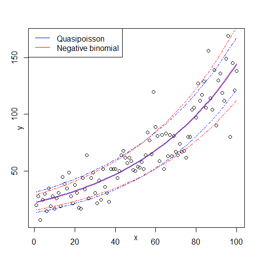
This difference in variance structure matters. The quasi-Poisson variance is linear in ; the negative binomial variance is quadratic. If your data show variance increasing faster than the mean at higher counts, the negative binomial may be a better fit.
Estimation and Interpretation
Estimation methods:
- The quasi-Poisson model is estimated via quasi-likelihood, which doesn't require a full distributional assumption. It maximizes a quasi-likelihood function that depends only on the mean-variance relationship. The dispersion parameter is typically estimated from the Pearson chi-square statistic divided by the residual degrees of freedom.
- The negative binomial model is estimated via maximum likelihood, since it specifies a complete probability distribution. Both coefficients and are estimated simultaneously.
Interpreting coefficients:
Regression coefficients in both models have the same interpretation as in Poisson regression. A coefficient represents the change in for a one-unit increase in , holding other variables constant.
Exponentiating gives you an incidence rate ratio (IRR):
An IRR of 1.25 means the expected count increases by 25% for each one-unit increase in that predictor. The key difference from Poisson regression is that the standard errors (and therefore confidence intervals and p-values) are adjusted for overdispersion, making inference more honest.
Assessing model fit:
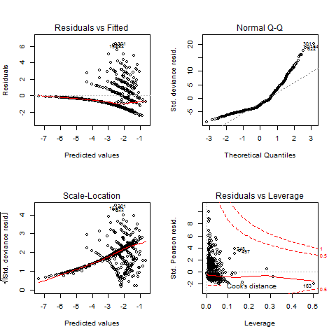
- Deviance and Pearson chi-square statistics evaluate overall goodness of fit. For a well-fitting model, these should be roughly equal to the residual degrees of freedom.
- Deviance residuals and Pearson residuals help you spot outliers and check assumptions. Plot them against fitted values and look for patterns.
Modeling Overdispersion
Quasi-Poisson Model
The quasi-Poisson approach is pragmatic. You keep the Poisson log-linear structure but inflate the standard errors by a factor of . This corrects inference without committing to a specific distribution.
Strengths:
- Flexible. Works across a range of overdispersion patterns.
- Simple to implement (in R, just change
family = poissontofamily = quasipoissoninglm()). - Point estimates of coefficients are identical to Poisson; only the standard errors change.
Limitations:
- No full probability model, so you can't compute likelihoods. This means AIC and likelihood ratio tests are unavailable.
- You can't use the model to generate predicted probability distributions for new observations.
Negative Binomial Model
The negative binomial approach commits to a distributional assumption, which buys you more tools when that assumption holds.
Strengths:
- Full probability model, so AIC, BIC, and likelihood ratio tests are all available.
- You can generate predicted probabilities and simulate from the fitted model.
- Often fits better when variance increases quadratically with the mean.
Limitations:
- More restrictive. If the true variance structure doesn't match , the model can be misspecified.
- Slightly more complex to fit (in R, use
glm.nb()from theMASSpackage).
Quasi-Poisson vs Negative Binomial
Comparison of Models
| Feature | Quasi-Poisson | Negative Binomial |
|---|---|---|
| Distributional assumption | None (mean-variance only) | Full negative binomial |
| Variance function | (linear) | (quadratic) |
| Overdispersion parameter | ||
| Estimation method | Quasi-likelihood | Maximum likelihood |
| AIC / likelihood ratio tests | Not available | Available |
| Predicted probabilities | Not available | Available |
| Coefficient estimates | Same as Poisson | Different from Poisson |
One subtle but important point: quasi-Poisson and Poisson give you the same coefficient estimates; only the standard errors differ. Negative binomial estimation changes the coefficient estimates themselves because it's fitting a different likelihood.
Choosing Between Models
There's no single rule, but here are practical guidelines:
-
Start with a Poisson model and check for overdispersion. Compute the ratio of the Pearson chi-square to the residual degrees of freedom. If it's substantially greater than 1, overdispersion is present.
-
For moderate overdispersion where your main goal is correct inference on regression coefficients, the quasi-Poisson model is often sufficient and simpler.
-
For substantial overdispersion, or when you need a full probability model (for prediction, simulation, or model comparison via AIC), use the negative binomial.
-
Compare variance structures. Plot the raw variance against the mean across groups in your data. If the relationship looks linear, quasi-Poisson may be more appropriate. If it looks quadratic, lean toward negative binomial.
-
Watch for zero-inflation. If your data have far more zeros than either model predicts, neither quasi-Poisson nor negative binomial will fix the problem. Consider zero-inflated Poisson (ZIP) or zero-inflated negative binomial (ZINB) models instead.
Model Selection for Overdispersion
Factors to Consider
- Degree of overdispersion: Mild overdispersion ( around 1.5–2) can often be handled by quasi-Poisson. Severe overdispersion may need negative binomial.
- Variance-mean relationship: Linear suggests quasi-Poisson; quadratic suggests negative binomial.
- Presence of excess zeros: Neither model is designed for zero-inflation.
- Research objectives: Do you need predicted probabilities, or just adjusted coefficient estimates?
Selection Criteria
For the negative binomial model, you can use standard model comparison tools:
- AIC and BIC balance fit against complexity. Lower values indicate a better trade-off.
- A likelihood ratio test comparing the Poisson model (nested within the negative binomial when ) directly tests whether the overdispersion parameter is needed. A significant result favors the negative binomial.
For the quasi-Poisson model, since no likelihood exists, you rely on:
- The estimated (values much greater than 1 confirm overdispersion).
- Residual plots and goodness-of-fit diagnostics.
When both models are candidates, fit both and compare residual patterns. If the negative binomial fits well and you value having AIC and predicted distributions, it's usually the stronger choice. If you just need robust standard errors and want minimal assumptions, quasi-Poisson does the job.