4.2 Detecting Outliers and Influential Observations

Outliers and Influential Observations

Defining Outliers and Influential Observations

Not all unusual data points cause the same problems in regression. It helps to distinguish between two categories:

• Outliers are observations whose response value ($y$) falls far from the value predicted by the model. They show up as large residuals.
• Influential observations are points that disproportionately affect the regression results. Removing a single influential point noticeably changes the estimated coefficients, fitted values, or model fit statistics.

A point can be an outlier without being influential, and a high-leverage point can be influential without being an obvious outlier in the $y$-direction. The key distinction is leverage vs. influence: leverage describes how far a point's predictor value ($x$) sits from the center of the predictor space, while influence describes how much that point actually changes the fitted model.

Outliers and influential observations can arise from measurement errors, data entry mistakes, or genuine extreme values in the population. Either way, they need to be identified and addressed, because ignoring them can produce biased or misleading regression results.

Consequences of Outliers and Influential Observations

• Biased coefficients: Outliers can pull the fitted regression line toward themselves, distorting slope and intercept estimates.
• Shifted regression line: High-leverage points sit at extreme $x$-values and can act like a pivot, tilting the line toward or away from the bulk of the data.
• Inflated residual variance: Even a single outlier can increase $MSE$, which widens confidence intervals and reduces the precision of all coefficient estimates.
• Violated assumptions: Outliers can create non-normal residual distributions, undermining the validity of $t$-tests and $F$-tests. They can also introduce heteroscedasticity (non-constant variance), which invalidates standard errors.

Identifying Outliers and Influential Observations

Visual Diagnostic Tools

Plots are your first line of defense. Each one targets a different kind of unusual observation:

• Residuals vs. fitted values plot: Points with unusually large positive or negative residuals stand out vertically. This is the primary tool for spotting outliers in the response variable.
• Residuals vs. predictor plot: Similar idea, but plotted against $x$ instead of $\hat{y}$. This helps reveal whether outliers cluster at particular predictor values.
• Scatterplot of $y$ vs. $x$: In simple linear regression, a basic scatterplot can reveal points that are far from the cloud of data in either the $x$- or $y$-direction (bivariate outliers).
• Normal Q-Q plot of residuals: Points that deviate sharply from the diagonal line indicate residuals that don't follow a normal distribution, often caused by outliers.

Numerical Diagnostic Measures

Visual tools catch the obvious cases. Numerical measures give you precise cutoffs.

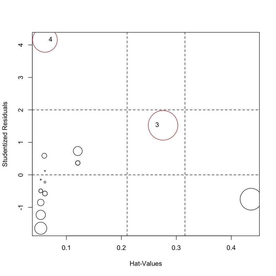
Leverage ($h_{ii}$) measures how far observation $i$'s predictor value is from the mean of all predictor values.

• Leverage values range from $1/n$ to 1. Values near 1 mean the point has extreme pull on the fitted line.
• The average leverage across all observations is $p/n$, where $p$ is the number of parameters (including the intercept) and $n$ is the sample size.
• A common rule of thumb: flag points with $h_{ii} > 2p/n$.
• High leverage alone doesn't mean a point is influential. It means the point could be influential if its $y$-value doesn't conform to the pattern set by the rest of the data.

Cook's Distance ($D_i$) combines residual size and leverage into a single measure of overall influence.

• It quantifies how much all the fitted values change when observation $i$ is deleted from the model.
• Observations with $D_i > 4/(n - p)$ are commonly flagged as influential. Some texts use $D_i > 1$ as a more conservative threshold.

DFFITS measures the change in the predicted value $\hat{y}_i$ when observation $i$ is removed.

• Flag observations where $|\text{DFFITS}_i| > 2\sqrt{p/n}$.
• This tells you how much a single point shifts its own predicted value.

DFBETAS measures the change in each individual regression coefficient when observation $i$ is removed.

• Flag observations where $|\text{DFBETAS}_{j,i}| > 2/\sqrt{n}$ for coefficient $j$.
• Unlike Cook's distance, DFBETAS pinpoints which coefficient a particular observation is affecting.

Impact of Outliers on Regression Results

Biased Coefficient Estimates

Outliers pull the regression line toward themselves. In simple linear regression, a single point far from the data cloud can change both the slope and intercept substantially. This leads to coefficient estimates that misrepresent the relationship for the majority of the data, potentially reversing the apparent direction or magnitude of an effect.

Inflated Residual Variance

Because OLS squares the residuals, a single large residual contributes disproportionately to $MSE$. The result is larger standard errors for all coefficients, wider confidence intervals, and reduced power to detect real relationships. In other words, one bad point can make your entire model look less precise than it actually is.

Compromised Model Assumptions

• Normality: Outliers create heavy tails or skewness in the residual distribution. This invalidates the $t$- and $F$-tests that depend on normally distributed errors, producing unreliable $p$-values.
• Homoscedasticity: Outliers can introduce or mask non-constant variance. If the residual spread changes across the range of fitted values, standard errors and confidence intervals become untrustworthy.

Handling Outliers in Regression Models

Investigating the Source of Outliers

Before doing anything else, figure out why the point is unusual:

1. Check for data entry errors or measurement mistakes. A misplaced decimal point can create a dramatic outlier.
2. Consult domain knowledge. Is this value plausible given the context of the study?
3. If the outlier results from a correctable error, fix it. If the data is clearly erroneous and cannot be corrected, removal is justified.

The goal is to distinguish between "this point is wrong" and "this point is real but extreme." Your handling strategy depends entirely on which case you're in.

Robust Regression Techniques

When outliers are genuine observations, robust regression methods reduce their influence without deleting data:

• Least Absolute Deviation (LAD) regression minimizes the sum of $|e_i|$ instead of $e_i^2$. Because it doesn't square residuals, large residuals don't dominate the objective function the way they do in OLS.
• M-estimation iteratively reweights observations, assigning smaller weights to points with large residuals. This downweights outliers automatically while still using all the data.

These techniques produce more stable coefficient estimates when the data contains genuine extreme values.

Variable Transformations

Sometimes a transformation of $y$ or $x$ reduces the severity of outliers by compressing the scale:

• Log transformation works well for positively skewed variables (e.g., income, population). It pulls in extreme right-tail values.
• Square root transformation is useful for right-skewed, non-negative variables (e.g., counts, areas). It's a milder compression than the log.

Transformations can simultaneously stabilize variance, improve residual normality, and reduce outlier influence. However, they change the interpretation of the model, so you need to be comfortable working on the transformed scale.

Sensitivity Analysis and Reporting

A sensitivity analysis lets you assess how much the outliers actually matter:

1. Fit the model with all observations included.
2. Refit the model excluding the flagged outliers or influential points.
3. Compare coefficient estimates, standard errors, $R^2$, and conclusions between the two fits.
4. If the results change substantially, the outliers are driving your conclusions and you need to address them explicitly.

Transparency matters. In your write-up:

• State which diagnostic criteria you used (e.g., Cook's distance > $4/(n-p)$, leverage > $2p/n$).
• Report the sensitivity analysis results so readers can judge for themselves.
• Justify your chosen approach (correction, removal, robust method, or transformation) based on the study context, not just convenience.