6.2 Interpreting Multiple Regression Coefficients

Regression Coefficients in Multiple Regression

Multiple regression coefficients tell you how each independent variable relates to the dependent variable while accounting for every other predictor in the model. Each coefficient captures the direction and magnitude of that variable's unique effect, which is essential for understanding which factors actually drive changes in your outcome.

Getting the interpretation right requires attention to a few things: multicollinearity between predictors, the range of your observed data, and whether your model includes all the relevant variables. Standardized coefficients become useful when you need to compare predictors measured on different scales.

Interpretation of Individual Coefficients

Each regression coefficient represents the change in the dependent variable for a one-unit increase in that predictor, holding all other independent variables constant. This "holding constant" part is what distinguishes multiple regression from running separate simple regressions.

• The sign tells you the direction of the relationship:
  • Positive: as the predictor increases, the dependent variable increases
  • Negative: as the predictor increases, the dependent variable decreases
• The magnitude (absolute value) tells you the strength:
  • Larger absolute values mean a bigger change in the dependent variable per unit change in the predictor
  • Smaller absolute values mean a smaller change

The coefficients carry the original units of your variables, which makes them directly interpretable. If your dependent variable is salary in dollars and one predictor is years of experience, a coefficient of 2,500 means each additional year of experience is associated with a $2,500 increase in salary, holding other predictors constant.

Two key assumptions underlie this interpretation:

• Linearity: the change in the dependent variable is the same for every one-unit change in the predictor, regardless of where you are on the scale
• Additivity: the effects of the independent variables combine by simple addition, meaning one predictor's effect doesn't depend on the value of another (unless you explicitly model interactions)

Assumptions and Limitations

The ceteris paribus assumption ("all else equal") is what lets you isolate each predictor's effect. In practice, you're relying on the model to statistically hold other variables constant, even though they may shift together in the real world.

Several things can undermine your coefficient interpretations:

• Multicollinearity occurs when independent variables are highly correlated with each other. It inflates the standard errors of your coefficients, making estimates unstable and hard to interpret. If two predictors share most of their variance, the model struggles to separate their individual contributions. In severe cases, methods like ridge regression or principal component regression can help.
• Extrapolation beyond observed data is risky. Your coefficients describe relationships within the range of data you actually collected. A linear relationship that holds between 0 and 10 years of experience may not hold at 40 years.
• Omitted variable bias arises when you leave out a relevant predictor that's correlated with one or more included predictors. The coefficients of the included variables absorb the omitted variable's effect, producing biased estimates. This is a model specification problem covered more broadly in this unit.

Unstandardized vs. Standardized Coefficients

Unstandardized Coefficients

Unstandardized coefficients (often labeled $b$) come straight from the regression on your original variables. They tell you the predicted change in $Y$ for a one-unit increase in $X_j$, in the original measurement units.

This makes them easy to interpret in context. A coefficient of 3.2 on a predictor measured in hours means "each additional hour is associated with a 3.2-unit increase in the outcome." The tradeoff is that you can't directly compare coefficients across predictors measured on different scales. A coefficient of 3.2 for hours and 0.004 for income in dollars doesn't mean hours matter more; the units are completely different.

Standardized Coefficients

Standardized coefficients (often labeled $\beta$) come from converting all variables to z-scores before running the regression. You standardize by subtracting the mean and dividing by the standard deviation:

$z = \frac{x - \bar{x}}{s}$

After this transformation, every variable has a mean of 0 and a standard deviation of 1. The resulting coefficients are unit-free and represent the change in $Y$ (in standard deviations) for a one-standard-deviation change in $X_j$.

For example, a standardized coefficient of 0.5 means that a one-standard-deviation increase in that predictor is associated with a 0.5-standard-deviation increase in the outcome. Because all predictors are now on the same scale, you can compare their absolute values to gauge relative strength.

The downside: standardized coefficients are less intuitive for practical communication. Telling someone "a one-SD increase in education predicts a 0.4-SD increase in income" is less concrete than "each additional year of education predicts $4,200 more in annual income."

Choosing Between Them

• Use unstandardized coefficients when you want practical, real-world interpretation in original units
• Use standardized coefficients when you want to compare the relative strength of predictors on different scales
• Reporting both is common and gives the most complete picture

Whichever you report, be explicit about which type you're presenting so readers don't misinterpret the results.

Predictor Importance from Coefficients

Assessing Relative Importance

Comparing the absolute values of standardized coefficients is the most straightforward way to rank predictor importance within a given model. A predictor with $|\beta| = 0.8$ has a stronger association with the outcome than one with $|\beta| = 0.2$, assuming both are in the same model.

But statistical significance and practical significance aren't the same thing. A predictor can be statistically significant (small p-value) yet have a tiny effect that doesn't matter in practice. Always evaluate whether the size of the effect is meaningful given your research context and domain knowledge.

Limitations and Considerations

• Multicollinearity makes relative importance rankings unreliable. When predictors share substantial variance, their individual coefficients become sensitive to small changes in the data or model. The coefficients may bounce around across samples even if the overall model is stable.
• Coefficients don't establish causation. A large standardized coefficient means a strong statistical association within your model, not that changing that predictor will cause a change in the outcome. Causal claims require theoretical justification or experimental design, not just regression output.
• Relative importance depends on what's in the model. Adding or removing a predictor can shift the coefficients of the remaining variables, sometimes substantially. This happens because the "holding constant" interpretation changes whenever the set of control variables changes. Always interpret importance rankings in the context of the specific model you've estimated.

Partial Regression Coefficients

Concept and Interpretation

In multiple regression, every coefficient is technically a partial regression coefficient. "Partial" means it captures the relationship between one predictor and the outcome after removing the influence of all other predictors in the model.

You can think of it this way: a partial regression coefficient answers the question, "If two observations have the same values on every other predictor, how much does the outcome differ per unit difference in this predictor?"

For example, if the partial coefficient for study hours is 0.5 in a model that also includes class attendance and prior GPA, it means each additional study hour is associated with a 0.5-unit increase in the outcome, among students who have the same attendance and prior GPA.

This is what makes multiple regression powerful. It lets you assess each variable's unique contribution to the outcome, net of the other variables.

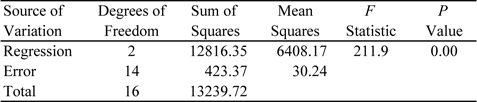
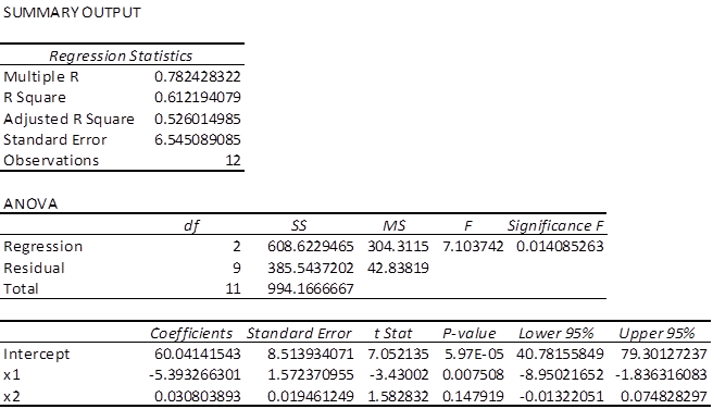
Hypothesis Testing and Significance

You can test whether each partial coefficient differs significantly from zero, which tells you whether that predictor adds unique explanatory power beyond the other variables.

The testing process works as follows:

1. State the null hypothesis: $H_0: \beta_j = 0$ (the predictor has no unique effect)
2. The regression software computes a t-statistic for each coefficient: $t = \frac{b_j}{SE(b_j)}$
3. Compare the resulting p-value to your chosen significance level (commonly 0.05)
4. If $p < \alpha$, reject the null and conclude the predictor has a statistically significant unique effect

t-tests handle individual coefficients. F-tests handle groups of coefficients simultaneously, which is useful when you want to test whether a set of related predictors (say, a group of dummy variables for a categorical variable) jointly contributes to the model.

A few things to keep in mind:

• A significant partial coefficient means the predictor contributes information beyond what the other predictors already explain. A non-significant result doesn't mean the variable is unrelated to the outcome; it may just be redundant with other predictors in the model.
• Statistical significance depends heavily on sample size. With large samples, even trivially small effects can be significant. Always consider the magnitude of the coefficient alongside its p-value.
• Practical significance matters. A coefficient that's statistically significant but substantively tiny may not warrant attention in your analysis, depending on the research question.