9.2 Feedback control

Feedback control is the strategy chemical engineers use to keep a process at its target by measuring what's actually happening and adjusting inputs accordingly. It's the foundation of safe, stable plant operation, and you'll see it applied everywhere from reactor temperature to pipeline flow rates.

Feedback Control Systems in Chemical Processes

Principles and Operation

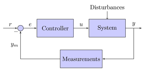
A feedback control system works by continuously monitoring a process output and correcting the input to hold a desired value called the setpoint. Four main components make this happen:

• Process: The physical operation being controlled (a reactor, a heat exchanger, etc.)
• Sensor / measuring device: Measures the controlled variable (temperature, pressure, flow rate) and sends a signal to the controller
• Controller: Compares the measured value to the setpoint, calculates the error, and determines what corrective action is needed
• Final control element (actuator): Receives the controller's signal and physically adjusts the manipulated variable (e.g., opening or closing a valve, changing heater output)

These components form a closed loop: the process output feeds back into the input side, so the system is always self-correcting. The key distinction here is between the controlled variable (what you're trying to keep at the setpoint, like temperature) and the manipulated variable (what the controller actually changes to get there, like coolant flow rate). Keeping these two straight will help you read block diagrams and troubleshoot loops much more easily.

Closed-Loop Operation

In closed-loop operation, the controller constantly watches for any gap between the measured value and the setpoint. When a deviation appears, the controller acts to shrink that gap.

This is what makes feedback control powerful. Even if unexpected disturbances hit the process (a sudden change in feed temperature, for instance), the loop detects the effect on the output and compensates automatically. The controller doesn't need to know why the output changed; it just sees the error and responds.

Common examples in chemical engineering:

• Reactor temperature control: A thermocouple measures temperature, and a control valve adjusts coolant or steam flow to hold the setpoint.
• pH control in neutralization: A pH sensor monitors the stream, and pumps adjust acid or base addition to maintain the target pH.

One limitation worth noting: because feedback control only reacts after the output has already deviated, there's always some lag. The system can't prevent a disturbance from affecting the process; it can only correct for it once the sensor picks up the change. This is why feedforward control (covered separately) is sometimes paired with feedback control for especially sensitive processes.

Block Diagrams of Feedback Control Loops

Main Components and Their Representations

Block diagrams are the standard way to visualize a control loop. Each component gets its own block, and arrows show how signals flow between them.

• The process block has an input (the manipulated variable) and an output (the controlled variable).
• The sensor block converts the physical measurement into a signal the controller can read (e.g., a thermocouple converting temperature to a voltage). This block also accounts for any measurement dynamics or lag introduced by the sensor itself.
• The controller block takes in the error signal and outputs a corrective command. This is often a PID controller or a programmable logic controller (PLC).
• The actuator block translates the controller's command into a physical change (e.g., a control valve adjusting flow, a variable-speed drive changing pump speed).

A typical block diagram arranges these in a loop: setpoint enters at the summing junction, the error feeds into the controller, the controller output goes to the actuator, the actuator adjusts the process, the process output goes to the sensor, and the sensor signal feeds back to the summing junction. Disturbances are usually shown as a separate arrow entering the process block, since they affect the output independently of the manipulated variable.

Signal Flow and Summing Junctions

Arrows on the diagram show the direction information travels through the loop. A key feature is the summing junction, drawn as a circle with a plus/minus sign.

The summing junction is where the setpoint and the measured value meet. It subtracts the measured signal from the setpoint to produce the error signal:

$e(t) = \text{setpoint} - \text{measured value}$

That error signal is what the controller acts on. If $e(t)$ is positive, the measured value is below the setpoint; if negative, it's above. For example, in a reactor temperature loop, the thermocouple signal is subtracted from the desired temperature setpoint at the summing junction, and the resulting error tells the controller whether to increase or decrease heating.

When you're reading or drawing these diagrams, trace the signal all the way around the loop to make sure the signs are correct. A sign error in the diagram flips the loop from negative feedback to positive feedback, which would drive the process away from the setpoint instead of toward it.

Negative Feedback for Process Stability

Concept and Mechanism

Negative feedback means the controller pushes the manipulated variable in the opposite direction of the error. This is what creates stability.

If a reactor's temperature rises above the setpoint, the controller reduces heat input (or increases cooling). If the temperature drops below the setpoint, the controller increases heat input. The corrective action always opposes the deviation, which drives the system back toward the setpoint.

By contrast, positive feedback would amplify the error: a temperature increase would cause even more heating, pushing the system further from the setpoint. Positive feedback is almost never desirable in process control and leads to instability.

Importance in Chemical Processes

Chemical processes are often sensitive to small changes. An exothermic reactor, for example, can experience thermal runaway if temperature isn't tightly controlled. In thermal runaway, a small temperature increase speeds up the reaction rate, which releases more heat, which raises the temperature further. Without negative feedback, this self-reinforcing cycle can escalate to dangerous conditions.

Negative feedback catches these disturbances early and corrects them before they grow. Two practical examples:

• Exothermic reactor temperature: Negative feedback keeps the reactor at the optimal temperature for product quality and prevents runaway. The controller increases coolant flow as soon as the temperature begins to creep up.
• Wastewater pH control: Discharge regulations often require pH within a narrow band (e.g., 6.0 to 9.0). Negative feedback adjusts acid or base dosing to meet those limits even as the incoming stream composition varies.

Performance Metrics for Feedback Control Systems

Steady-State Error and Response Time

Once you have a feedback loop running, you need to evaluate how well it performs. Two fundamental metrics:

• Steady-state error: The difference between the setpoint and the controlled variable after the system has fully settled. A good controller keeps this small (ideally zero). Integral action in a PID controller is specifically designed to eliminate steady-state error. A proportional-only controller, by contrast, will almost always leave some residual offset.
• Response time: How long it takes the controlled variable to reach its new steady-state value after a setpoint change or disturbance. Shorter is generally better, but pushing for very fast response can cause other problems like overshoot or oscillation.

Other Performance Indicators

Several additional metrics help engineers evaluate and tune control loops:

• Overshoot: The maximum amount the controlled variable exceeds the setpoint during a transient response, usually expressed as a percentage. For example, 10% overshoot on a 100°C setpoint means the temperature temporarily hits 110°C.
• Settling time: The time for the controlled variable to stay within a specified tolerance band (commonly ±5% or ±2%) around the setpoint.
• Rise time: The time for the controlled variable to go from its initial value to a specified fraction (typically 90%) of the final steady-state value. Rise time and overshoot tend to trade off against each other: a faster rise time often means more overshoot.
• Decay ratio: The ratio of the amplitude of one oscillation peak to the next. A decay ratio less than 1 means oscillations are shrinking, which indicates stability. A common design target is a decay ratio of about 0.25 (quarter-decay), meaning each successive peak is one-quarter the height of the previous one.

These metrics are directly tied to controller tuning. Adjusting the parameters of a PID controller (proportional gain, integral time, derivative time) changes the tradeoffs between response speed, overshoot, and stability. There's no single "best" tuning for all situations. A reactor with a risk of thermal runaway might prioritize minimal overshoot, while a flow control loop on a non-hazardous stream might tolerate more overshoot in exchange for faster response. Engineers use these performance indicators to find the right balance for each specific process.