7.1 Diffusion and Fick's law

Mass transfer principles

Mass transfer describes how substances move from regions of high concentration to regions of low concentration. This concept shows up everywhere in chemical engineering, from separation processes to reactor design, so building a solid intuition for it now will pay off throughout the course.

Fundamentals of mass transfer and diffusion

Mass transfer is the net movement of a substance driven by a concentration gradient. Diffusion is a specific type of mass transfer that happens at the molecular level: molecules bounce around randomly due to their kinetic energy, and the statistical result is net movement from high to low concentration.

• Diffusion is spontaneous. It doesn't require external energy input because it's driven by the second law of thermodynamics. Molecules naturally spread out, increasing entropy.
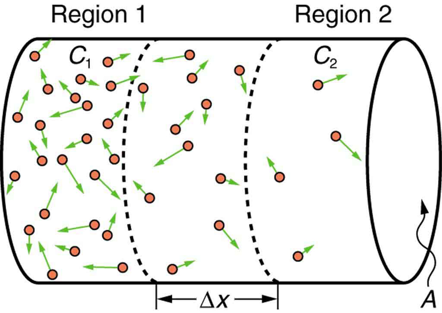
• The rate of diffusion is proportional to the concentration gradient. A steeper gradient means more molecules crossing a given plane per unit time, so diffusion happens faster.

Steady-state and unsteady-state diffusion

These are the two main categories of diffusion problems you'll encounter:

• Steady-state diffusion: The concentration profile doesn't change with time. The flux at any point stays constant, which makes the math much simpler (you only need Fick's first law).
• Unsteady-state diffusion: The concentration profile evolves over time. The flux depends on both position and time, so you need Fick's second law, which introduces partial differential equations.

Most real-world processes start as unsteady-state and eventually approach steady-state if conditions are held constant long enough.

Diffusion rate calculation

Fick's first law of diffusion

Fick's first law connects the diffusive flux to the concentration gradient. In one dimension:

$J = -D \frac{dC}{dx}$

where:

• $J$ = diffusive flux (mol/m²·s), the amount of substance passing through a unit area per unit time
• $D$ = diffusivity or diffusion coefficient (m²/s)
• $\frac{dC}{dx}$ = concentration gradient (mol/m⁴)

The negative sign matters. Concentration decreases in the direction of diffusion, so $\frac{dC}{dx}$ is negative in that direction. The negative sign in the equation makes $J$ positive in the direction of net mass flow (from high to low concentration).

Fick's first law applies across phases:

• Gases: pollutant spreading through air (typical $D \sim 10^{-5}$ m²/s)
• Liquids: salt dissolving into water (typical $D \sim 10^{-9}$ m²/s)
• Solids: dopant atoms diffusing into a silicon wafer (typical $D \sim 10^{-14}$ m²/s or smaller)

Notice how diffusivity drops by many orders of magnitude from gases to solids. That pattern reflects how tightly packed the molecules are in each phase.

Fick's second law of diffusion

Fick's second law describes how concentration at a given point changes over time. For one-dimensional diffusion with constant diffusivity:

$\frac{\partial C}{\partial t} = D \frac{\partial^2 C}{\partial x^2}$

This equation says: the rate of concentration change at a point depends on the curvature of the concentration profile at that point. Where the profile curves sharply, concentration changes quickly.

To solve Fick's second law, you need:

1. Initial condition: the concentration distribution at $t = 0$
2. Boundary conditions: what happens at the edges of your system (fixed concentration, no-flux, or a combination)

For simple geometries and boundary conditions, analytical solutions exist. The most common one you'll see is the error function solution for a semi-infinite medium with a constant surface concentration. For more complex cases, numerical methods like finite difference or finite element are used.

Diffusion influencing factors

Concentration gradient and diffusivity

The concentration gradient is the driving force, but the diffusion coefficient $D$ determines how easily molecules actually move through a given medium.

Several factors affect $D$:

• Temperature: Higher temperature means more kinetic energy, so molecules move faster and $D$ increases. For gases, $D$ is roughly proportional to $T^{1.5}$ to $T^{1.75}$.
• Molecular size and shape: Smaller, more spherical molecules diffuse faster because they encounter less resistance from surrounding molecules.
• Pressure (mainly for gases): Higher pressure packs molecules closer together, reducing $D$.

Medium properties and multi-component systems

The medium itself plays a big role:

• Viscosity: Higher viscosity means more drag on diffusing molecules, which lowers $D$. The Stokes-Einstein equation captures this relationship for dilute liquid solutions: $D$ is inversely proportional to viscosity.
• Porosity and tortuosity: In porous materials (like catalysts or membranes), molecules can't travel in straight lines. They follow winding paths through pores, so the effective diffusivity is lower than the free-space value. A common correction is $D_{eff} = D \cdot \frac{\varepsilon}{\tau}$, where $\varepsilon$ is porosity and $\tau$ is tortuosity.

In multi-component systems, diffusion gets more complicated. The presence of other species creates additional molecular interactions (attractive or repulsive forces) and competition for space. The Maxwell-Stefan equations handle these interactions and are more general than Fick's law, though Fick's law remains a good approximation for dilute binary systems.

Steady-state vs unsteady-state diffusion

Solving steady-state diffusion problems

Because the concentration profile doesn't change with time, steady-state problems use Fick's first law directly. For a one-dimensional slab with constant diffusivity:

$J = -D \frac{\Delta C}{\Delta x}$

where $\Delta C$ is the concentration difference across the slab and $\Delta x$ is its thickness.

Example: Gas diffuses through a 2 mm thick membrane. The concentration on one side is 0.5 mol/L and on the other side is 0.1 mol/L. If $D = 1.0 \times 10^{-10}$ m²/s:

1. Calculate the gradient: $\frac{\Delta C}{\Delta x} = \frac{0.5 - 0.1}{0.002} = 200$ mol/m⁴ (after unit conversion)

2. Apply Fick's first law: $J = (1.0 \times 10^{-10})(200) = 2.0 \times 10^{-8}$ mol/m²·s

The key assumption is that concentrations on both sides stay constant (perhaps because fresh gas is continuously supplied and removed).

Solving unsteady-state diffusion problems

When concentrations change with time, you need Fick's second law. The general approach:

1. Write out Fick's second law for your geometry (planar, cylindrical, or spherical).
2. Define your initial condition (concentration everywhere at $t = 0$).
3. Define your boundary conditions (what's happening at the surfaces).
4. Solve analytically if the geometry and conditions are simple enough; otherwise, use numerical methods.

Common examples:

• A drug tablet dissolving into surrounding fluid, where the drug concentration at the tablet surface decreases over time
• Heat treating a metal part, where the surface concentration of a diffusing element (like carbon in carburization) is held constant while the interior concentration gradually increases

For a semi-infinite solid with a suddenly imposed constant surface concentration, the analytical solution uses the error function:

$\frac{C(x,t) - C_0}{C_s - C_0} = 1 - \text{erf}\left(\frac{x}{2\sqrt{Dt}}\right)$

where $C_s$ is the surface concentration, $C_0$ is the initial concentration, and $\text{erf}$ is the error function (values are typically looked up in a table or computed). This solution is surprisingly useful for many practical problems, especially at short times before diffusion reaches the far boundary of the material.