2.3 Entropy Changes in Various Processes

Entropy Changes in Various Processes

Entropy changes let you quantify how far a process departs from the ideal reversible case and how much useful work potential is lost along the way. Mastering the entropy calculations for different process types is essential for applying the Second Law to real engineering systems.

This section covers entropy changes in reversible vs. irreversible processes, specific process types (isothermal, adiabatic, polytropic), entropy generation and its link to exergy destruction, and entropy balances for both closed and open systems.

Entropy Changes in Processes

Calculating Entropy Changes in Reversible and Irreversible Processes

Entropy is a state function, so its change depends only on the initial and final states, never on the path. This is what allows you to evaluate $\Delta S$ along any convenient reversible path between the same two end states, even if the actual process is irreversible.

For a reversible process, the entropy change is calculated directly from the heat transfer:

$\Delta S = \int \frac{\delta Q_{\text{rev}}}{T}$

where $\delta Q_{\text{rev}}$ is the differential reversible heat transfer and $T$ is the absolute temperature at the boundary where that transfer occurs.

For an irreversible process, the actual heat integral underestimates the entropy change:

$\Delta S > \int \frac{\delta Q}{T}$

The difference between the left and right sides is the entropy generated internally ($S_{\text{gen}}$). You still compute $\Delta S$ by choosing a reversible path between the same end states; the inequality tells you that the entropy transferred by heat alone doesn't account for all of the system's entropy increase.

How the surroundings respond:

• Reversible process: $\Delta S_{\text{surr}} = -\Delta S_{\text{sys}}$, so the net change for the universe is zero.
• Irreversible process: $\Delta S_{\text{surr}} < -\Delta S_{\text{sys}}$, so the universe experiences a net entropy increase.

The Second Law, stated concisely: for an isolated system, $\Delta S_{\text{iso}} \geq 0$, with equality only for reversible processes.

Entropy Changes in the Universe

The total entropy change of the universe is the sum of the system and surroundings contributions:

$\Delta S_{\text{univ}} = \Delta S_{\text{sys}} + \Delta S_{\text{surr}}$

• For a reversible process: $\Delta S_{\text{univ}} = 0$.
• For an irreversible process: $\Delta S_{\text{univ}} > 0$.

The magnitude of $\Delta S_{\text{univ}}$ is a direct measure of the process's irreversibility and the lost potential for doing useful work. A larger value means more work potential has been permanently degraded.

Common irreversible processes that increase universal entropy:

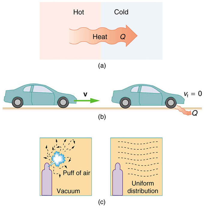
• Spontaneous heat transfer across a finite temperature difference (e.g., a 500 K block contacting a 300 K reservoir)
• Free expansion of a gas into an evacuated space ($Q = 0$, $W = 0$, yet entropy rises)
• Mixing of two different gases at the same $T$ and $P$
• Friction, viscous dissipation, and inelastic deformation

Entropy Changes for Specific Processes

Isothermal and Adiabatic Processes

Isothermal processes (constant $T$) simplify the entropy integral because temperature comes out of the integrand:

$\Delta S = \frac{Q}{T}$

For an ideal gas expanding or compressing isothermally, internal energy doesn't change ($\Delta U = 0$), so $Q = W$. Substituting the ideal-gas work expression gives:

$\Delta S = nR \ln \frac{V_2}{V_1}$

where $n$ is the number of moles and $R$ is the universal gas constant. An expansion ($V_2 > V_1$) produces a positive $\Delta S$; a compression produces a negative $\Delta S$ (entropy leaves via heat rejection).

Adiabatic processes have no heat transfer ($Q = 0$):

• Reversible adiabatic (isentropic): $\Delta S = 0$. This is the idealization used for turbines, compressors, and nozzles.
• Irreversible adiabatic: $\Delta S > 0$. Internal irreversibilities like friction, turbulence, or shock waves generate entropy even though no heat crosses the boundary. The entropy increase here equals $S_{\text{gen}}$ directly, since there's no entropy transfer term.

Polytropic Processes

A polytropic process follows the relation:

$PV^n = \text{constant}$

where $n$ is the polytropic exponent. By choosing different values of $n$, you recover several familiar processes as special cases:

For an ideal gas undergoing a general polytropic process, the entropy change can be written as:

$\Delta S = n_{\text{mol}} C_v \ln \frac{T_2}{T_1} + n_{\text{mol}} R \ln \frac{V_2}{V_1}$

where $n_{\text{mol}}$ is the number of moles (note: don't confuse this with the polytropic exponent $n$). If you already know the polytropic exponent and want to express everything in terms of temperature alone, you can use the polytropic $T$-$V$ relation to eliminate the volume ratio. For a constant-volume process specifically, the second term vanishes and you get $\Delta S = n_{\text{mol}} C_v \ln(T_2/T_1)$.

On a $P$-$V$ diagram, higher values of the polytropic exponent produce steeper process curves. On a $T$-$s$ diagram, the exponent determines whether the process line tilts left or right relative to the vertical isentropic line.

Entropy Generation in Systems

Causes and Effects of Entropy Generation

Every real process generates entropy. The main sources of irreversibility are:

• Friction and viscous dissipation (mechanical energy converted to thermal energy)
• Heat transfer across a finite temperature difference (the larger $\Delta T$, the more entropy generated)
• Unrestrained expansion (expansion against a pressure lower than the system pressure)
• Mixing of dissimilar substances
• Chemical reactions proceeding spontaneously

The Gouy-Stodola theorem connects entropy generation directly to lost work:

$W_{\text{lost}} = T_0 \, S_{\text{gen}}$

where $T_0$ is the ambient (dead-state) temperature. This is a powerful result: every unit of entropy generated costs you $T_0$ units of work that you can never recover. For a process at $T_0 = 300 \text{ K}$ that generates $S_{\text{gen}} = 0.5 \text{ kJ/K}$, the lost work is 150 kJ.

Minimizing entropy generation is the thermodynamic basis for improving efficiency. Practical strategies include reducing temperature differences in heat exchangers, minimizing pressure drops in piping, and staging compression with intercooling.

Exergy and Entropy Generation

Exergy (also called availability) is the maximum useful work obtainable from a system as it comes into equilibrium with its environment. Exergy destruction is the flip side of entropy generation:

$\dot{Ex}_{\text{dest}} = T_0 \, \dot{S}_{\text{gen}}$

This equation has the same form as Gouy-Stodola because exergy destruction is lost work potential. Performing an exergy analysis on each component of a system lets you pinpoint where the largest irreversibilities occur and rank them by magnitude.

Typical applications of exergy analysis:

• Power cycles (Rankine, Brayton): identify whether the boiler, turbine, condenser, or pump is the dominant source of loss
• Refrigeration cycles (vapor-compression, absorption): quantify compressor and throttling valve losses
• Heat exchangers: evaluate how much work potential is destroyed by the stream-to-stream $\Delta T$

Entropy Balance for Systems

Closed Systems

The entropy balance for a closed system (no mass crossing the boundary) is:

$\Delta S_{\text{sys}} = \int \frac{\delta Q}{T_{\text{boundary}}} + S_{\text{gen}}$

Reading this equation left to right: the system's entropy change equals the entropy transferred in by heat plus the entropy created internally.

• Reversible case: $S_{\text{gen}} = 0$, so $\Delta S_{\text{sys}}$ equals the heat-transfer integral exactly.
• Irreversible case: $S_{\text{gen}} > 0$, so the system's entropy rises by more than what heat transfer alone would produce.

When applying this to a problem, follow these steps:

1. Define the system boundary and identify all heat interactions.

2. Determine the boundary temperature(s) at which heat transfer occurs.

3. Calculate $\Delta S_{\text{sys}}$ from property tables or ideal-gas relations (state function, so use any convenient path).

4. Evaluate the heat-transfer integral $\int \delta Q / T_{\text{boundary}}$.

5. Solve for $S_{\text{gen}} = \Delta S_{\text{sys}} - \int \delta Q / T_{\text{boundary}}$.

6. Confirm $S_{\text{gen}} \geq 0$. A negative value signals an error in your calculation or an impossible process.

Open Systems

For an open (control volume) system, mass carries entropy across the boundary, so the balance gains inlet and outlet terms:

$\frac{dS_{\text{CV}}}{dt} = \sum_j \frac{\dot{Q}_j}{T_j} + \sum_i \dot{m}_i s_i - \sum_o \dot{m}_o s_o + \dot{S}_{\text{gen}}$

where:

• $\dot{Q}_j / T_j$ is the rate of entropy transfer by heat at each boundary location $j$
• $\dot{m}_i s_i$ and $\dot{m}_o s_o$ are entropy carried in and out by mass flow
• $\dot{S}_{\text{gen}}$ is the rate of entropy generation within the control volume

Steady-state simplification: When operating conditions don't change with time, $dS_{\text{CV}}/dt = 0$, and the equation reduces to:

$0 = \sum_j \frac{\dot{Q}_j}{T_j} + \sum_i \dot{m}_i s_i - \sum_o \dot{m}_o s_o + \dot{S}_{\text{gen}}$

This is the form you'll use most often for devices like turbines, compressors, heat exchangers, and nozzles. Combined with mass and energy balances, it gives you enough equations to solve for unknowns like exit states, heat transfer rates, or isentropic efficiencies.

A useful check: after solving, always verify that $\dot{S}_{\text{gen}} \geq 0$. If it comes out negative, either the assumed process violates the Second Law or there's an error in your setup.