4.3 Solving Systems Using Matrices

Augmented matrices for systems

more resources to help you study

practice questions

Representing systems of linear equations

A system of linear equations is two or more equations that share the same variables. An augmented matrix gives you a compact way to write such a system: the coefficients of the variables fill the main columns, and the constants from the right side of each equation go in one extra column at the end.

• Each row corresponds to one equation.
• Each of the first columns corresponds to one variable.
• The final column holds the constants.

When you set up the augmented matrix, make sure every equation lists the variables in the same order. If a variable is missing from an equation, its coefficient is 0.

Dimensions and structure of augmented matrices

For a system with $m$ equations and $n$ variables, the augmented matrix has $m$ rows and $n + 1$ columns.

For example, take this 2-equation, 2-variable system:

$2x + 3y = 5$ $4x - y = 3$

The augmented matrix is:

$\begin{bmatrix} 2 & 3 & 5 \\ 4 & -1 & 3 \end{bmatrix}$

This is a $2 \times 3$ matrix: 2 rows (one per equation) and 3 columns (2 variable columns + 1 constant column). A system with 3 equations and 3 variables would produce a $3 \times 4$ augmented matrix.

Solving systems with row operations

Elementary row operations

The goal is to transform the augmented matrix into a simpler form where you can read off the solution directly. There are three operations you're allowed to perform, and none of them change the solution set:

1. Swap two rows. (Interchange rows $R_i$ and $R_j$.)
2. Multiply a row by a nonzero constant. (Replace $R_i$ with $kR_i$, where $k \neq 0$.)
3. Add a multiple of one row to another. (Replace $R_i$ with $R_i + kR_j$.)

You use these operations to reach one of two target forms:

• Row-echelon form (REF): Every leading entry (first nonzero number in a row) sits to the right of the leading entry in the row above, and any all-zero rows are at the bottom.
• Reduced row-echelon form (RREF): Same as REF, but every leading entry is 1 and it's the only nonzero entry in its column.

RREF is the most useful because the solution can be read directly from the matrix.

Applying row operations strategically

A reliable strategy for reaching RREF:

1. Work column by column, left to right. For each column, get a leading 1 on the diagonal (swap rows or multiply if needed).
2. Use Type 3 operations to eliminate all other entries in that column (both below and above the leading 1).
3. Move to the next column and repeat.

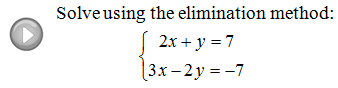
Worked example. Solve $2x + 3y = 5$, $4x - y = 3$.

Start with the augmented matrix:

$\begin{bmatrix} 2 & 3 & 5 \\ 4 & -1 & 3 \end{bmatrix}$

Step 1: Divide $R_1$ by 2 to get a leading 1.

$\begin{bmatrix} 1 & 3/2 & 5/2 \\ 4 & -1 & 3 \end{bmatrix}$

Step 2: Replace $R_2$ with $R_2 - 4R_1$ to eliminate the 4 below the leading 1.

$\begin{bmatrix} 1 & 3/2 & 5/2 \\ 0 & -7 & -7 \end{bmatrix}$

Step 3: Divide $R_2$ by $-7$ to get a leading 1 in the second row.

$\begin{bmatrix} 1 & 3/2 & 5/2 \\ 0 & 1 & 1 \end{bmatrix}$

Step 4: Replace $R_1$ with $R_1 - \frac{3}{2}R_2$ to eliminate the $3/2$ above the second leading 1.

$\begin{bmatrix} 1 & 0 & 1 \\ 0 & 1 & 1 \end{bmatrix}$

Read the solution: $x = 1$, $y = 1$.

Consistency and independence of systems

Determining consistency

After row-reducing, look at the bottom rows of the matrix to classify the system.

• Consistent: The system has at least one solution. No row reads $\begin{bmatrix} 0 & 0 & \cdots & 0 & c \end{bmatrix}$ where $c \neq 0$.
• Inconsistent: The system has no solution. At least one row translates to $0 = c$ (with $c \neq 0$), which is a contradiction.

For a 3-equation, 2-variable system, consider these two reduced forms:

Determining independence

Once you know a system is consistent, the next question is how many solutions it has.

• Independent: Exactly one solution. In RREF, every variable column has a leading 1 (a pivot).
• Dependent: Infinitely many solutions. At least one variable column lacks a pivot, meaning that variable is free and can take any value.

Interpreting solutions in context

Modeling real-world situations

Systems of equations show up whenever multiple conditions must be satisfied at the same time. The variables represent unknown quantities, and each equation captures a relationship between them.

For instance, suppose a bakery makes cakes and pies. If ingredients limit total production to 100 items and the bakery needs twice as many cakes as pies, you'd write:

$x + y = 100$ $x = 2y$

Here $x$ is the number of cakes and $y$ is the number of pies. Solving the augmented matrix gives the production plan that meets both constraints.

Interpreting solutions and their implications

Always check whether the mathematical answer makes sense in the real situation.

• A negative value for a quantity that must be positive (like a number of items) signals that the model's constraints may be unrealistic.
• No solution means the constraints contradict each other. In the bakery example, it might mean the ingredient limits and the demand ratio can't both be satisfied.
• Infinitely many solutions means there isn't enough information to pin down a single answer. Some quantities can vary freely, and you'd need an additional constraint to narrow things down.
• A unique solution means the constraints fully determine every unknown, which is usually the ideal outcome in applied problems.