Solving Systems of Equations

Defining Systems of Equations
A system of equations is a set of two or more equations that share the same variables, solved simultaneously to find their common solution(s). In this unit, you're mostly dealing with systems that pair a quadratic equation with a linear equation, though you can also have two quadratics together.
These systems can be solved algebraically (substitution or elimination) or graphically. Each method has its strengths depending on the problem.
Algebraic Methods for Solving Systems
Substitution is usually the go-to method for quadratic-linear systems. Here's how it works:
- Solve the linear equation for one variable (typically ).
- Substitute that expression into the quadratic equation, replacing .
- Simplify and solve the resulting quadratic equation (you'll get a single-variable quadratic).
- Plug your solution(s) back into the linear equation to find the corresponding value(s) of the other variable.
- Write your answer(s) as ordered pairs.
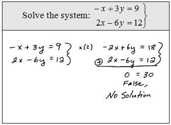
Elimination works best when both equations are already in the same form (for example, both solved for ). Set them equal to each other, then solve the resulting equation. This is really just a variation of substitution.
Example: Solve and .
Set them equal:
Rearrange:
Factor: , so or
Plug back in: when , ; when , Solutions: and
Graphical Solutions and the Discriminant
Graphically, the solutions to a system are the points of intersection of the two graphs. For a quadratic-linear system, there are three possible outcomes:
- Two intersection points → two real solutions
- One intersection point (the line is tangent to the parabola) → one real solution
- No intersection points → no real solutions
You can predict which case you're in without graphing. After substituting and simplifying to a single quadratic equation, check the discriminant ():
- → two real solutions
- → one real solution
- → no real solutions
Modeling with Quadratic Functions

Real-World Applications of Quadratic Functions
Quadratic functions show up whenever a quantity increases and then decreases (or vice versa) in a symmetric pattern. Common applications include projectile motion, area optimization, and revenue/profit modeling.
The key properties you'll use for modeling are the vertex (gives the maximum or minimum value), the axis of symmetry, the x-intercepts (zeros), and the concavity (whether the parabola opens up or down).
Projectile Motion
The standard projectile motion model is:
where is the acceleration due to gravity (approximately or ), is the initial velocity, and is the initial height.
For example, a ball thrown upward at 48 ft/s from ground level gives . Here's what the quadratic tells you:
- Vertex: The maximum height and the time it occurs. Use seconds. Plug back in: feet.
- Positive x-intercept: The time the projectile lands. Set and solve; here, seconds.
- The term (the constant) gives the launch height. In this case it's 0, meaning the ball was thrown from ground level.
Optimization Problems
Optimization problems ask you to find the maximum or minimum value of a quantity that can be modeled quadratically. The vertex always gives you the optimal value.
A classic example is the fencing problem: You have 60 meters of fencing and want to enclose the largest possible rectangular area against a wall (so you only need three sides of fencing). If is the width, the length is , and the area is:
Since , the parabola opens downward, so the vertex is a maximum. The optimal width is meters, giving a maximum area of square meters.
Applying Quadratic Functions
Problem-Solving with Quadratic Functions
When you encounter a word problem, follow these steps:
- Identify the variables. What quantity are you trying to optimize or solve for? What are the given constraints?
- Build the equation. Translate the relationships described in the problem into a quadratic function.
- Solve. Use the vertex formula, factoring, the quadratic formula, or graphing depending on what the problem asks.
- Interpret. Translate your mathematical answer back into the context of the problem, with units.
Interpreting Solutions and Considering Constraints
Not every mathematical solution makes sense in a real-world context. Always check your answers against the problem's constraints:
- Non-negative constraints: Time, length, and quantity can't be negative. If you get seconds as one solution for a projectile problem, discard it.
- Domain restrictions: A fencing problem where represents a width requires and also that the other dimensions remain positive.
- Discrete vs. continuous: If you're optimizing the number of items produced, your answer needs to be a whole number, even if the vertex gives you .
When presenting your solution, state your answer clearly, include units, and note any assumptions the model makes (e.g., ignoring air resistance in projectile motion).
Quadratic vs. Linear and Exponential Functions
Comparing Function Properties
Understanding how quadratic functions differ from linear and exponential functions helps you recognize which model fits a given situation.
| Property | Linear | Quadratic | Exponential |
|---|---|---|---|
| General form | |||
| Rate of change | Constant (slope ) | Varies (changes linearly) | Constant percent change |
| Graph shape | Straight line | Parabola | Curve (J-shape or decay) |
| Max/Min | None | Vertex (max if , min if ) | No max/min (has horizontal asymptote) |
How to tell them apart from a table of values: Calculate the first differences (change in ). If they're constant, it's linear. If the second differences are constant, it's quadratic. If the ratios of consecutive -values are constant, it's exponential.
Intercepts, Vertices, and End Behavior
- Y-intercept: For all three types, plug in . For linear, it's . For quadratic, it's . For exponential, it's (the initial value).
- X-intercepts: Linear functions have exactly one (unless horizontal). Quadratics can have 0, 1, or 2. Exponential functions with a horizontal asymptote at have no x-intercept (the curve approaches but never touches the axis).
End behavior is where these functions diverge most dramatically:
- Linear: One end goes to , the other to (unless slope is 0).
- Quadratic: Both ends go in the same direction. If , both ends rise toward . If , both ends fall toward .
- Exponential: One end approaches the horizontal asymptote, and the other end grows without bound (for growth) or the reverse (for decay).
A practical takeaway: for large values of , exponential growth will always eventually outpace quadratic growth, and quadratic growth will always eventually outpace linear growth. This matters when you're choosing which model best fits a real-world scenario over different time horizons.