12.3 Polar Coordinates and Complex Numbers in Trigonometric Form

Rectangular vs Polar Coordinates

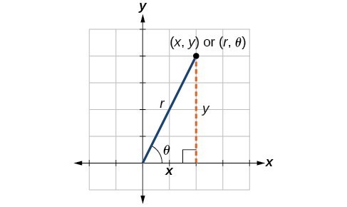
Rectangular coordinates $(x, y)$ describe a point using horizontal and vertical distances from the origin. Polar coordinates $(r, \theta)$ describe the same point using a distance $r$ from the origin and an angle $\theta$ measured from the positive $x$-axis. Both systems locate the same points; they just use different measurements to get there.

more resources to help you study

practice questions

Converting Between Coordinate Systems

Polar to rectangular is the more straightforward direction:

$x = r\cos\theta \qquad y = r\sin\theta$

Rectangular to polar requires more care:

$r = \sqrt{x^2 + y^2} \qquad \theta = \tan^{-1}\!\left(\frac{y}{x}\right)$

The catch with $\theta$: your calculator's $\tan^{-1}$ only returns values in $\left(-\frac{\pi}{2}, \frac{\pi}{2}\right)$, which covers Quadrants I and IV. If the point is in Quadrant II or III (meaning $x < 0$), you need to add $\pi$ to the calculator result to get the correct angle.

One more detail: the origin $(0, 0)$ in rectangular corresponds to $r = 0$ in polar, but the angle $\theta$ is undefined there since there's no unique direction from the origin to itself.

Comparing Coordinate Systems

• Rectangular coordinates work well for grid-like settings (maps, standard graphs, linear equations).
• Polar coordinates shine when a problem involves distance and direction from a central point (radar, circular motion, navigation).
• Some equations simplify dramatically in polar form. A circle centered at the origin is $x^2 + y^2 = a^2$ in rectangular but just $r = a$ in polar.

Graphing Polar Equations

Plotting Points and Curves

Polar equations have the form $r = f(\theta)$. To graph one:

1. Build a table of $\theta$ values, usually from $0$ to $2\pi$ (choose increments like $\frac{\pi}{6}$ or $30°$).
2. Calculate the corresponding $r$ for each $\theta$.
3. Plot each point $(r, \theta)$ on polar graph paper (or by converting to rectangular).
4. Connect the points with a smooth curve.

For example, to graph $r = 2\sin(3\theta)$, you'd evaluate $r$ at $\theta = 0°, 30°, 60°, \ldots, 330°$. This particular equation produces a rose curve with 3 petals.

Common polar curves you should recognize:

• Circles: $r = a$ (centered at origin) or $r = a\cos\theta$ / $r = a\sin\theta$ (passing through origin)
• Cardioids: $r = a(1 + \cos\theta)$ — heart-shaped, with a cusp at the origin
• Limaçons: $r = a + b\cos\theta$ — may have an inner loop if $b > a$
• Rose curves: $r = a\cos(n\theta)$ — $n$ petals if $n$ is odd, $2n$ petals if $n$ is even

Identifying Symmetry

Testing for symmetry saves you work when graphing because you only need to plot part of the curve and reflect the rest.

• Symmetry about the polar axis (horizontal axis): Replace $\theta$ with $-\theta$. If the equation is unchanged, the curve is symmetric about the polar axis.
• Symmetry about the origin: Replace $r$ with $-r$ (or equivalently, replace $\theta$ with $\theta + \pi$). If the equation is unchanged, the curve is symmetric about the origin.
• Symmetry about the line $\theta = \frac{\pi}{2}$ (vertical axis): Replace $\theta$ with $\pi - \theta$. If the equation is unchanged, the curve has vertical symmetry.

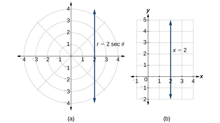
Note: an equation like $r = \frac{1}{\cos\theta}$ is actually the vertical line $x = 1$ in rectangular form. It's undefined at $\theta = \frac{\pi}{2}$ and $\theta = \frac{3\pi}{2}$ because $\cos\theta = 0$ there, producing vertical asymptotes in the polar graph.

Complex Numbers in Trigonometric Form

Representing Complex Numbers

Any complex number $z = a + bi$ can be rewritten in trigonometric (polar) form:

$z = r(\cos\theta + i\sin\theta)$

Here $r$ is the modulus (the distance from the origin to the point $(a, b)$ on the complex plane) and $\theta$ is the argument (the angle from the positive real axis).

The conversion formulas are the same as rectangular-to-polar:

$r = \sqrt{a^2 + b^2} \qquad \theta = \tan^{-1}\!\left(\frac{b}{a}\right) \text{ (with quadrant adjustments)}$

You may also see the shorthand cis notation: $r\;\text{cis}\;\theta = r(\cos\theta + i\sin\theta)$.

Euler's formula provides yet another equivalent form: $e^{i\theta} = \cos\theta + i\sin\theta$, so $z = re^{i\theta}$. This is useful for understanding why multiplication and division rules work the way they do.

Geometric Interpretation

On the complex plane, the modulus $r$ tells you how far the number is from the origin, and the argument $\theta$ tells you the direction. For instance, $2(\cos\frac{\pi}{3} + i\sin\frac{\pi}{3})$ sits 2 units from the origin at a $60°$ angle. This geometric view makes operations like multiplication and finding roots much more intuitive.

Operations on Complex Numbers

Multiplication and Division

Trigonometric form turns multiplication and division into simple arithmetic on the moduli and arguments.

Multiplication: Multiply the moduli, add the arguments.

$r_1(\text{cis}\;\theta_1) \cdot r_2(\text{cis}\;\theta_2) = r_1 r_2\;\text{cis}(\theta_1 + \theta_2)$

Division: Divide the moduli, subtract the arguments.

$\frac{r_1(\text{cis}\;\theta_1)}{r_2(\text{cis}\;\theta_2)} = \frac{r_1}{r_2}\;\text{cis}(\theta_1 - \theta_2)$

If your resulting angle falls outside $[0, 2\pi)$, add or subtract $2\pi$ to bring it back into the principal range.

Powers and Roots (De Moivre's Theorem)

De Moivre's Theorem is the key result here. For any complex number $z = r(\cos\theta + i\sin\theta)$ and positive integer $n$:

$z^n = r^n(\cos(n\theta) + i\sin(n\theta))$

You raise the modulus to the $n$th power and multiply the argument by $n$. This is far faster than multiplying $z$ by itself $n$ times in rectangular form.

Finding $n$th roots uses the same theorem in reverse. The $n$th roots of $z = r(\cos\theta + i\sin\theta)$ are:

$z_k = \sqrt[n]{r}\left(\cos\frac{\theta + 2k\pi}{n} + i\sin\frac{\theta + 2k\pi}{n}\right), \quad k = 0, 1, 2, \ldots, n-1$

This gives exactly $n$ distinct roots, evenly spaced around a circle of radius $\sqrt[n]{r}$.

Steps to find $n$th roots:

1. Write the complex number in trigonometric form $r(\cos\theta + i\sin\theta)$.
2. Compute $\sqrt[n]{r}$ for the new modulus.
3. For $k = 0$, the first root has argument $\frac{\theta}{n}$.
4. Each successive root ($k = 1, 2, \ldots$) adds $\frac{2\pi}{n}$ to the argument.

The geometric spacing of roots is a useful check: if your roots aren't evenly distributed around the circle, something went wrong in the calculation.