3.3 Linear Programming

Linear programming is a method for finding the best possible outcome (like maximum profit or minimum cost) given a set of constraints written as linear inequalities. It pulls together everything you've learned about graphing inequalities and systems of equations, then applies it to optimization problems where you need to make the smartest choice within real-world limits.

more resources to help you study

practice questions

Formulating Linear Programs

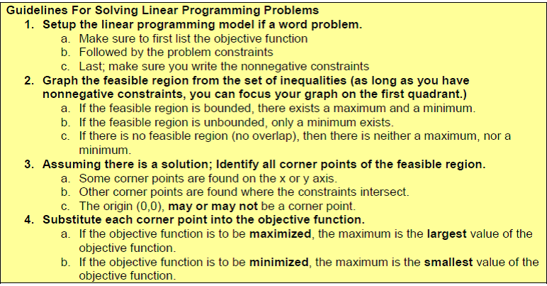
Every linear programming problem has three components: decision variables, constraints, and an objective function. Setting these up correctly is the most important step.

Identifying Decision Variables

Decision variables are the unknowns you're solving for. They represent the quantities you get to choose. In an Honors Algebra II context, you'll typically work with two variables ($x$ and $y$) so you can graph the problem on a coordinate plane.

• $x$ might represent the number of units of Product A to manufacture
• $y$ might represent the number of units of Product B to manufacture

The whole point of the problem is figuring out what values of $x$ and $y$ give you the best result.

Defining Constraints

Constraints are the rules your solution must follow, written as linear inequalities (or occasionally equations). They come from real-world limitations like budget, time, materials, or minimum requirements.

• Resource limits restrict how much you can use: "You have at most 40 hours of labor per week" becomes something like $2x + 5y \leq 40$
• Minimum requirements set a floor: "You must produce at least 3 units of Product B" becomes $y \geq 3$
• Non-negativity constraints almost always apply: $x \geq 0$ and $y \geq 0$, because you can't produce a negative number of items

Each constraint carves away part of the coordinate plane. Together, they define the region where valid solutions live.

Formulating the Objective Function

The objective function is the expression you want to maximize or minimize. It's a linear function of your decision variables:

$Z = ax + by$

The coefficients $a$ and $b$ represent how much each variable contributes to your goal. For example, if Product A earns 5 dollars profit per unit and Product B earns 3 dollars per unit, your objective function is:

$Z = 5x + 3y$

You then either maximize or minimize $Z$ depending on the problem (maximize profit, minimize cost, etc.).

Solving Linear Programs Graphically

Determining the Feasible Region

The feasible region is the set of all points $(x, y)$ that satisfy every constraint at the same time. Here's how to find it:

1. Graph each constraint as a boundary line. Use a solid line for $\leq$ or $\geq$, and a dashed line for strict inequalities.
2. Shade the correct side of each line. For $\leq$, shade below/left; for $\geq$, shade above/right. (Test a point like $(0, 0)$ if you're unsure.)
3. Identify the overlap. The feasible region is where all the shaded areas intersect. It's typically a polygon.

For example, the constraints $x \geq 0$, $y \geq 0$, and $x + y \leq 10$ produce a triangular feasible region with vertices at $(0, 0)$, $(10, 0)$, and $(0, 10)$.

If there's no overlapping region, the system has no feasible solution.

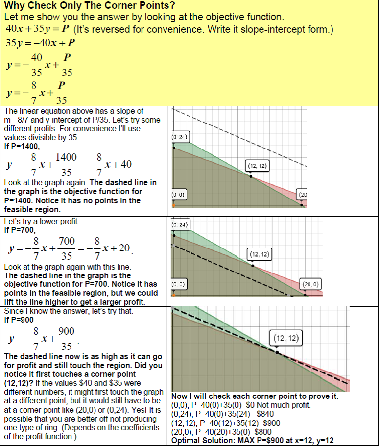
Finding the Optimal Solution

This is where the Corner Point Theorem (also called the Vertex Theorem) comes in: if an optimal solution exists, it occurs at a vertex (corner point) of the feasible region. That fact saves you from testing infinitely many points.

1. Find all vertices of the feasible region. These are points where boundary lines intersect. Solve pairs of equations to get exact coordinates.
2. Evaluate the objective function at each vertex. Plug each vertex into $Z = ax + by$.
3. Compare values. The vertex that gives the largest $Z$ is your maximum; the smallest is your minimum.

Interpreting Linear Programming Results

Understanding the Optimal Solution

Once you've found the optimal vertex, translate it back into the context of the problem. The coordinates tell you what to do, and the objective function value tells you how well it works.

• The values of $x$ and $y$ are your optimal decisions: "Produce 10 units of Product A and 0 units of Product B."
• The value of $Z$ is your optimized outcome: "This yields a maximum profit of 30 dollars."

Always check that your answer makes sense in context. If the problem asks about whole items and you get a fractional answer, note that the true optimum may need rounding (though for this course, most problems are designed to produce integer solutions at the vertices).

Conducting Sensitivity Analysis

Sensitivity analysis asks: What happens if the numbers change slightly?

• Changing coefficients in the objective function can shift which vertex is optimal. If the profit per unit of Product A rises from 3 to 4 dollars, a different corner point might become the best choice.
• Changing a constraint (like getting more hours of labor) can expand or shrink the feasible region, creating new vertices and potentially a better optimal value.
• Binding constraints are the ones that the optimal solution sits right on. These are the constraints that, if loosened, would most improve your result.

This type of analysis helps you understand which limitations matter most and how stable your solution is if conditions shift.

Limitations of Linear Programming Models

Linear programming is useful, but it rests on assumptions that don't always hold perfectly in the real world. For an Honors Algebra II course, you should be aware of these:

Linearity Assumption

All relationships (objective function and constraints) must be linear. If doubling production doesn't exactly double cost, or if there are economies of scale, the real relationship is nonlinear and can't be modeled directly with LP. For this course, problems will always give you linear relationships, but recognize that this is a simplification.

Continuity Assumption

LP assumes decision variables can be any real number (including fractions like $x = 4.7$). In practice, you often need whole-number answers: you can't build 4.7 cars. Problems requiring integer solutions technically need integer programming, though in this course you'll mostly encounter problems where the vertices happen to be integers.

Certainty Assumption

LP assumes you know all the coefficients exactly. In reality, costs fluctuate, demand is uncertain, and supply can be disrupted. The sensitivity analysis discussed above is a first step toward dealing with this, but true uncertainty requires more advanced methods beyond this course.

Model Simplification

Every LP model is a simplified version of reality. It might ignore setup costs, assume constant production rates, or leave out constraints that are hard to quantify. The quality of your answer depends on how well the model captures the actual situation. A technically correct solution to a poorly built model won't be very helpful.