Zero-Padding for DFT/FFT
Concept and Purpose of Zero-Padding
Zero-padding means appending zeros to the end of a time-domain signal before computing the DFT/FFT. This increases the total number of samples, which in turn produces more finely spaced frequency bins in the output. The result is a smoother, more detailed picture of the frequency spectrum.
A common practical reason to zero-pad is to bring the signal length up to a power of 2 (e.g., from 1000 samples to 1024), since the FFT algorithm runs most efficiently at those lengths.
One thing that trips people up: zero-padding does not add new spectral information. It interpolates between the existing frequency points, giving you a denser sampling of the same underlying spectrum. Think of it as increasing the pixel count on an image you already have. The picture doesn't get sharper in terms of actual detail, but it does get smoother and easier to read.
Relationship between Frequency Resolution and Signal Length
The spacing between adjacent frequency bins is given by:
where is the sampling frequency and is the total number of samples (including any appended zeros).
As increases, shrinks, meaning the frequency bins are packed more closely together. This lets you better distinguish between nearby frequency components in the plot. But remember: the true resolving power of the DFT still depends on the original signal duration , where is the number of actual (non-zero) samples. Zero-padding refines the grid you're sampling the spectrum on; it doesn't improve the fundamental ability to separate two genuinely distinct frequencies.
Frequency Resolution Enhancement with Zero-Padding
Applying Zero-Padding for Improved Frequency Resolution
Here's the step-by-step process:
-
Decide on your target length . This might be chosen to hit a specific , or simply to reach the next power of 2.
-
Calculate how many zeros to append: , where is the original signal length.
-
Append the zeros to the end of the time-domain signal.
-
Compute the DFT/FFT on the zero-padded signal of length .
For example, suppose you have a signal sampled at Hz with samples. The original bin spacing is:
If you zero-pad to :
You now have twice as many frequency bins, giving a smoother spectral curve.
Interpreting the Zero-Padded Frequency Spectrum
The extra frequency bins from zero-padding are interpolated values, not new frequency content. Keep that in mind when reading the output: a sharp-looking peak doesn't necessarily mean you've resolved two close frequencies that were previously merged. It may just be a more finely drawn version of the same single peak.
That said, the denser bin spacing is genuinely useful for:
- Locating peak frequencies more precisely (the true peak is less likely to fall between bins)
- Producing cleaner-looking spectral plots for visualization
- Reducing the "picket fence" effect, where you miss energy that falls between widely spaced bins
Windowing Effects on Frequency Spectrum
Spectral Leakage and the Need for Windowing
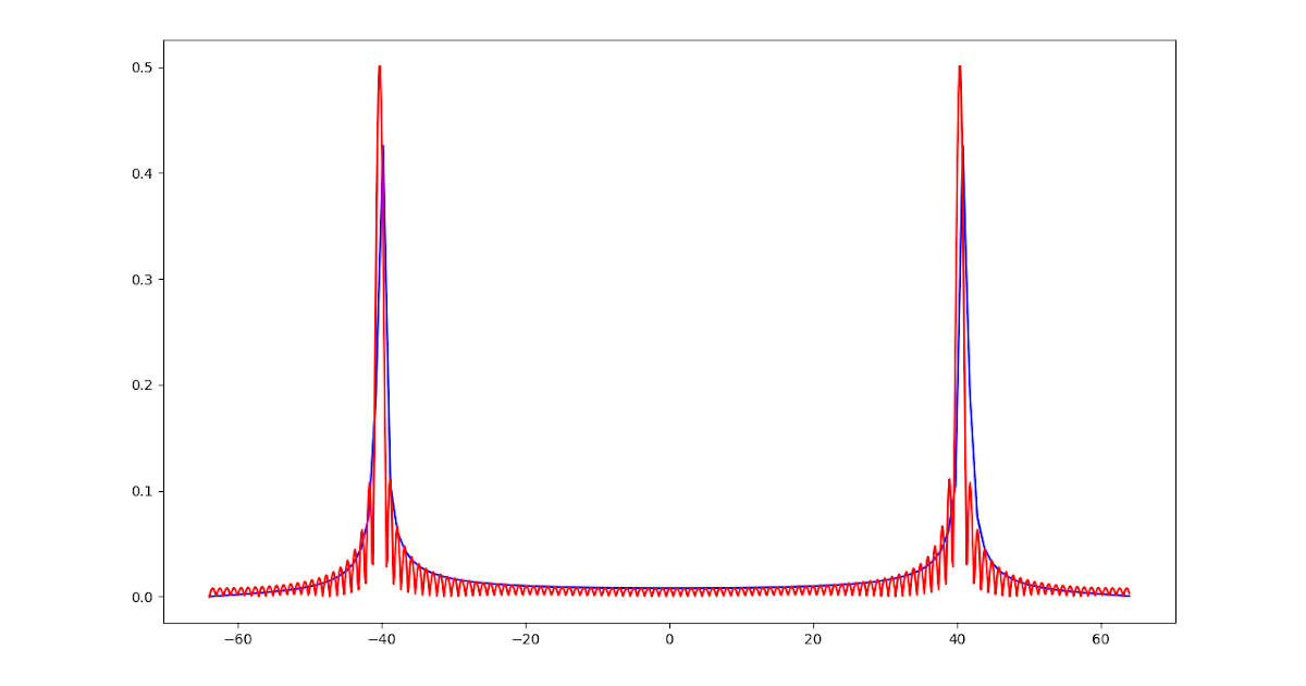
The DFT assumes the input signal is one period of a periodic sequence. When the signal isn't perfectly periodic within the analysis window, discontinuities appear at the boundaries where the signal "wraps around." These discontinuities cause the signal's energy to spread across many frequency bins instead of staying concentrated where it belongs. This spreading is called spectral leakage.
Consider a simple example: a pure sinusoid at exactly 100 Hz, sampled so that the analysis window contains an integer number of cycles. The DFT output will show a clean spike at 100 Hz. Now shift the frequency slightly so the window captures a non-integer number of cycles. Suddenly the energy smears across neighboring bins, and the clean spike turns into a broad hump with sidelobes. Nothing changed about the signal; the mismatch between the signal period and the window length created the leakage.
Windowing addresses this by multiplying the time-domain signal by a function that smoothly tapers toward zero at both ends. This reduces the boundary discontinuities and suppresses the sidelobes in the frequency domain.
Characteristics and Trade-offs of Different Window Functions
Every window function represents a trade-off between two competing goals:
- Narrow main lobe → better frequency resolution (ability to separate close frequencies)
- Low side lobes → less spectral leakage (less energy bleeding into distant bins)
Here's how the most common windows compare:
| Window | Main Lobe Width | Side Lobe Level | Best For |
|---|---|---|---|
| Rectangular (none) | Narrowest | Highest (~-13 dB) | Signals already periodic in the window |
| Hann | Moderate | Low (~-31 dB) | General-purpose spectral analysis |
| Hamming | Moderate | Lower (~-42 dB) | Similar to Hann, slightly better sidelobe suppression |
| Blackman | Wide | Very low (~-58 dB) | Signals with weak components near strong ones |
| Kaiser | Adjustable | Adjustable | Flexible; tuned via parameter |
The Hann window is a solid default choice for most situations. It gives up some frequency resolution compared to the rectangular window but dramatically cuts down on leakage.
Window Function Selection for Spectral Estimation
Factors to Consider When Selecting a Window Function
Your choice of window depends on what matters most for your application:
- If your signal is already periodic in the window (or very close to it), the rectangular window works fine and gives you the best frequency resolution.
- If you need to detect weak frequency components near strong ones, you need low sidelobes. Blackman or Kaiser (with high ) will keep the strong component's leakage from masking the weak one.
- If you want a general-purpose balance, Hann or Hamming windows are the standard go-to choices.
- If you need precise control over the trade-off, the Kaiser window lets you dial in the balance by adjusting its parameter. Higher means lower sidelobes but a wider main lobe.
Applying Window Functions and Analyzing the Frequency Spectrum
The application process is straightforward:
- Choose a window function based on the criteria above.
- Generate the window of the same length as your signal (most signal processing libraries have built-in functions for this).
- Multiply the time-domain signal by the window, sample by sample:
- Compute the DFT/FFT on the windowed signal .
- Interpret the spectrum, keeping in mind that the main lobe is wider than it would be with no window, but the sidelobes are suppressed.
One practical detail: windowing reduces the overall signal energy (since you're multiplying parts of the signal by values less than 1). If you're measuring absolute magnitudes, you may need to apply a coherent gain correction to compensate.
Zero-padding and windowing work well together. A typical workflow is: apply a window to reduce leakage, then zero-pad to get finer frequency bin spacing. The window handles the leakage problem; the zero-padding gives you a smoother, more readable spectrum.