9.2 Time-Frequency Localization

Time-Frequency Localization

Definition and Importance

Time-frequency localization refers to the ability of an analysis method to simultaneously capture when something happens in a signal and at what frequency. These two pieces of information live in different domains, and most classical tools only give you one at a time.

• Time domain representations show how a signal varies over time, letting you identify features like onset, duration, and decay (e.g., the envelope of a sound or segments in speech).
• Frequency domain representations reveal spectral content, showing which frequency components are present and how strong they are (e.g., harmonic structure or formant frequencies in vowels).

Time-frequency analysis methods like the Short-Time Fourier Transform (STFT) and wavelet transforms try to give you both simultaneously. They do this by using analysis windows or basis functions that are localized in both domains to varying degrees. Which method you pick depends on the signal you're working with and how you want to balance temporal vs. spectral resolution.

Limitations and Trade-offs

Perfect localization in both time and frequency is impossible. The Heisenberg uncertainty principle sets a hard floor on the simultaneous resolution you can achieve in both domains. Sharpen one, and the other necessarily blurs.

• Shorter windows give better time resolution but poorer frequency resolution. This is useful for transient detection or capturing impulse responses.
• Longer windows give better frequency resolution but poorer time resolution. This suits steady-state analysis or pitch estimation.

The choice of window size and shape directly controls where you sit on this trade-off curve. There's no way to cheat it; you can only choose the trade-off that best fits your application.

Heisenberg Uncertainty Principle

Formulation and Interpretation

The Heisenberg uncertainty principle originates in quantum mechanics, where it states that the product of uncertainties in a particle's position and momentum is always at least $\hbar/2$. Signal processing borrows the same mathematical structure.

In our context, the principle says that the product of time resolution $\Delta t$ and frequency resolution $\Delta f$ is bounded from below:

$\Delta t \cdot \Delta f \geq \frac{1}{4\pi}$

Here $\Delta t$ and $\Delta f$ are the standard deviations of the signal's energy distribution in time and frequency, respectively. A Gaussian window actually achieves equality in this bound, making it the "optimal" window in the uncertainty-product sense. Every other window shape yields a strictly larger product.

Implications for Signal Analysis

This bound has direct consequences for how you design and interpret time-frequency representations:

• The time-bandwidth product $\Delta t \cdot \Delta f$ is fixed at best, so any gain in one dimension costs you in the other.
• Your choice of analysis window (Gaussian, Hann, rectangular, etc.) determines exactly where you land on the trade-off.
• When reading a spectrogram or scalogram, you need to keep the resolution limits in mind. A "blob" in a spectrogram isn't necessarily a single event; it may be a sharp event smeared by limited frequency resolution, or a narrow-band component smeared by limited time resolution.

Wavelets vs. Fourier Basis Functions

Fourier Basis Functions

Fourier basis functions are complex sinusoids $e^{j2\pi ft}$ that extend infinitely in time. This gives them perfect frequency localization (each basis function sits at exactly one frequency) but zero time localization.

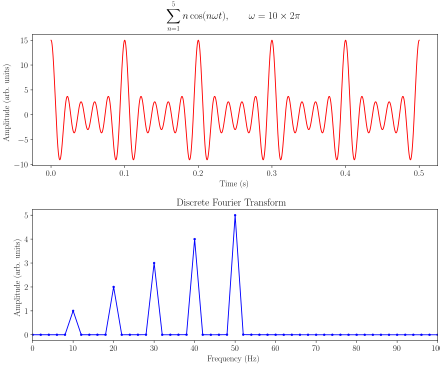
The Fourier transform decomposes a signal into a weighted sum of these sinusoids, producing a frequency spectrum or power spectral density. That's powerful for stationary signals whose statistical properties don't change over time (pure tones, periodic waveforms). But because the transform integrates over all time, it cannot tell you when a particular frequency was present. Artifacts like spectral leakage and the Gibbs phenomenon also arise when the signal doesn't fit neatly into the infinite-sinusoid model.

Wavelets

Wavelets are short, oscillatory functions localized in both time and frequency. Instead of analyzing a signal with infinite sinusoids, you analyze it with translated and scaled copies of a single mother wavelet (e.g., Haar, Morlet, Daubechies).

The key advantage is adaptive resolution:

• At high frequencies (small scales): the wavelet is compressed in time, giving fine time resolution but coarser frequency resolution. This is exactly what you want for catching transients and sharp edges.
• At low frequencies (large scales): the wavelet stretches out, giving fine frequency resolution but coarser time resolution. This suits slowly varying components where you care more about precise pitch than precise timing.

This adaptive behavior is the foundation of multi-resolution analysis. A companion scaling function (father wavelet) captures the low-frequency approximation of the signal, while the mother wavelet captures high-frequency detail at each scale. The wavelet transform produces approximation coefficients (from the scaling function) and detail coefficients (from the wavelet function) at each level.

Wavelets are especially well-suited for non-stationary signals like speech, music, and biomedical data, where frequency content changes over time. Their good time localization lets them detect transient events such as discontinuities, clicks, or abrupt changes that Fourier methods tend to smear out.