3.3 Frequency Spectrum Analysis

Signal Frequency Spectrum

Fourier Transform Basics

The Fourier Transform lets you decompose any continuous signal into a sum of sinusoids at different frequencies. Instead of looking at how a signal changes over time, you get to see which frequencies are present and how strong each one is.

The continuous-time Fourier Transform (CTFT) is defined as:

$X(f) = \int_{-\infty}^{\infty} x(t)e^{-j2\pi ft} \, dt$

Here, $x(t)$ is your time-domain signal, $f$ is frequency in Hz, and $j$ is the imaginary unit ($j^2 = -1$). The output $X(f)$ is generally complex-valued, meaning it encodes both amplitude and phase information at every frequency.

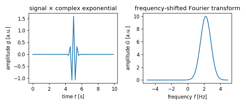
The key idea: multiplying by $e^{-j2\pi ft}$ and integrating essentially "tests" how much of frequency $f$ is present in the signal. If the signal contains a strong component at that frequency, the integral produces a large value.

Discrete Fourier Transform (DFT) and Fast Fourier Transform (FFT)

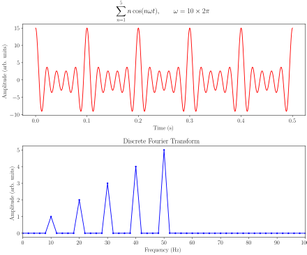
Since this unit focuses on continuous signals, the CTFT is the main tool. But in practice, you'll almost always compute frequency spectra numerically using the Discrete Fourier Transform (DFT):

$X[k] = \sum_{n=0}^{N-1} x[n] \, e^{-j(2\pi/N)kn}$

where $N$ is the number of samples and $k$ is the frequency index (corresponding to frequency $f_k = k/N \cdot f_s$, with $f_s$ being the sampling rate).

The Fast Fourier Transform (FFT) isn't a different transform. It's an efficient algorithm for computing the DFT that reduces computational complexity from $O(N^2)$ to $O(N \log N)$. For a signal with $N = 10{,}000$ samples, that's roughly a 2,500x speedup. This is what makes real-time spectrum analysis feasible in audio, image, and video processing.

The Inverse Fourier Transform reverses the process, reconstructing the time-domain signal from its frequency-domain representation. This means no information is lost in the transform: you can go back and forth between domains freely.

Magnitude and Phase Spectra

Components of the Frequency Spectrum

Because $X(f)$ is complex-valued, it's typically split into two real-valued functions:

• Magnitude spectrum $|X(f)|$: the amplitude of each frequency component. This tells you how much of each frequency is in the signal. It's often plotted on a logarithmic scale in decibels ($\text{dB} = 20\log_{10}|X(f)|$) so you can visualize both very strong and very weak components on the same plot.
• Phase spectrum $\angle X(f)$: the phase angle of each frequency component, typically in radians ($-\pi$ to $\pi$) or degrees ($-180°$ to $180°$). This tells you the timing offset of each sinusoidal component relative to a reference.

Together, magnitude and phase fully describe the signal in the frequency domain. You need both to reconstruct the original time-domain signal.

Interpreting Magnitude and Phase Spectra

Reading the magnitude spectrum:

• Peaks correspond to frequencies where the signal carries the most energy. For a periodic signal, you'll see a peak at the fundamental frequency and additional peaks at its harmonics (integer multiples).
• The overall shape tells you whether the signal is narrowband (energy concentrated around a few frequencies) or wideband (energy spread across many frequencies).

Reading the phase spectrum:

• A constant phase shift across all frequencies means the signal is simply shifted in time.
• A linear phase vs. frequency relationship indicates a pure time delay with no distortion. This is the ideal behavior for filters that need to preserve waveform shape.
• A nonlinear phase relationship means different frequency components are delayed by different amounts, causing dispersion (the waveform shape changes as it propagates or passes through a system).

Phase is often harder to interpret visually than magnitude, but it matters enormously. Two signals can have identical magnitude spectra yet sound or look completely different because of their phase relationships.

Bandwidth, Center Frequency, and Resolution

Bandwidth and Center Frequency

Bandwidth is the range of frequencies over which a signal has significant energy. There are several conventions for defining "significant," but the most common is the 3 dB bandwidth: the frequency range where the magnitude spectrum stays within 3 dB of its peak value (i.e., above $|X(f)|_{\max} / \sqrt{2}$).

For example, if a bandpass signal has significant energy between 900 Hz and 1100 Hz, its bandwidth is 200 Hz.

Center frequency is the midpoint of that band. In the example above, the center frequency is 1000 Hz. Center frequency is especially important in communications, where signals are often shifted to specific carrier frequencies for modulation and demodulation.

Spectral Resolution

Spectral resolution is your ability to distinguish between two closely spaced frequency components. It's governed by a fundamental relationship:

$\Delta f = \frac{1}{T}$

where $T$ is the duration of the signal (or observation window). If you observe a signal for 0.1 seconds, your frequency resolution is 10 Hz, meaning you can't tell apart two sinusoids that are less than 10 Hz apart.

This creates a direct trade-off:

• Longer observation time → better frequency resolution, but you lose the ability to track how the spectrum changes over time.
• Shorter observation time → poorer frequency resolution, but you can see how the spectrum evolves.

This is a form of the time-frequency uncertainty principle, and it's one of the most important practical constraints in spectrum analysis. Applications like vibration analysis and radar processing often require careful choices about observation window length to balance time and frequency resolution.

Frequency Spectrum Analysis in Applications

Signal Processing Domains

Audio and speech processing relies heavily on spectrum analysis. An equalizer, for instance, works by modifying the magnitude spectrum in specific frequency bands. Speech recognition systems extract spectral features (like formant frequencies, which are the resonant peaks of the vocal tract) to distinguish between phonemes. Audio compression formats like MP3 use spectral analysis to identify and discard frequency components that human hearing is less sensitive to.

Communications systems use spectrum analysis to characterize channel bandwidth, design filters for separating overlapping signals, and evaluate spectral efficiency (how many bits per second you can transmit per Hz of bandwidth). Modulation schemes like FM and OFDM are best understood in the frequency domain, where you can see how information is encoded across different frequency bands.

Radar systems exploit the Doppler effect: a moving target shifts the frequency of a reflected signal. By analyzing the frequency spectrum of the return signal, radar can estimate target velocity, separate moving targets from stationary clutter, and improve signal-to-noise ratio through matched filtering.

Biomedical Signal Processing

Biomedical signals have characteristic frequency signatures that make spectrum analysis a natural diagnostic tool.

• EEG (brain signals): Different brain states produce activity in distinct frequency bands. Alpha waves (8-13 Hz) appear during relaxed wakefulness, beta waves (13-30 Hz) during active thinking, and delta waves (0.5-4 Hz) during deep sleep. Spectrum analysis enables sleep stage classification and brain-computer interfaces.
• ECG (heart signals): The frequency content of an ECG can reveal arrhythmias and other cardiac abnormalities. Heart rate variability analysis, which examines low-frequency vs. high-frequency power in the heart rate signal, provides information about autonomic nervous system function.

In all these biomedical applications, frequency-domain techniques also help with noise reduction by allowing you to filter out frequency bands that contain interference (like 50/60 Hz power line noise) while preserving the physiologically relevant components.