1.4 Linear Time-Invariant (LTI) Systems

Properties of LTI Systems

Linear Time-Invariant (LTI) systems are the backbone of signal processing. They're predictable and mathematically tractable because they follow two rules: linearity and time-invariance. Once you know an LTI system's impulse response, you can figure out its output for any input. That single fact is what makes them so powerful.

Linearity and Time-Invariance

Linearity means the system obeys superposition and scaling. If you feed in a weighted combination of inputs, the output is the same weighted combination of the individual outputs:

$T\{a_1 x_1(t) + a_2 x_2(t)\} = a_1 y_1(t) + a_2 y_2(t)$

where $y_1(t) = T\{x_1(t)\}$ and $y_2(t) = T\{x_2(t)\}$. This bundles two sub-properties together:

• Superposition (additivity): The response to a sum of inputs equals the sum of individual responses.
• Scaling (homogeneity): Scaling the input by a constant scales the output by the same constant.

Time-invariance means the system behaves the same regardless of when you apply the input. If $x(t)$ produces $y(t)$, then a shifted input $x(t - t_0)$ produces the shifted output $y(t - t_0)$ for any time shift $t_0$. The system's internal rules don't change over time.

Together, these two properties guarantee that the output can be expressed as a superposition of scaled and shifted impulse responses, which leads directly to convolution.

Impulse Response and System Characterization

An LTI system is fully characterized by its impulse response $h(t)$, which is the output when the input is a unit impulse $\delta(t)$. Because any signal can be decomposed into a sum of scaled, shifted impulses, knowing $h(t)$ lets you compute the output for any input via convolution.

Two additional properties matter for practical systems:

• Stability (BIBO): A system is bounded-input, bounded-output stable if every bounded input produces a bounded output. The condition is $\int_{-\infty}^{\infty} |h(t)|\, dt < \infty$. In other words, the impulse response must be absolutely integrable.
• Causality: A system is causal if the output at any time depends only on current and past inputs, never future ones. This requires $h(t) = 0$ for $t < 0$.

Most real-world systems need to be both stable and causal. When you see an impulse response, check these two conditions first.

Impulse and Step Responses

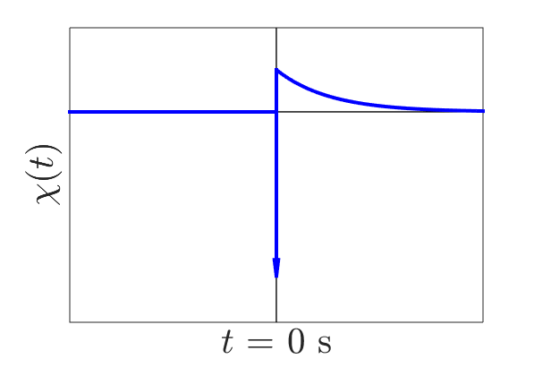
Impulse Response

The impulse response $h(t)$ is the output when you feed a unit impulse $\delta(t)$ into the system. For discrete-time systems, it's the output sequence $h[n]$ when the input is the unit impulse $\delta[n]$.

Why does this single response characterize the entire system? Any input signal can be written as a continuous sum (integral) of shifted, scaled impulses. Linearity and time-invariance then let you express the output as the same continuous sum of shifted, scaled impulse responses. That's exactly what convolution computes.

Step Response

The step response $s(t)$ is the output when the input is the unit step function $u(t)$. For discrete-time systems, it's the output when the input is $u[n]$.

The step response and impulse response are directly related. Since the unit step is the running integral of the impulse, the step response is the running integral of the impulse response:

$s(t) = \int_{-\infty}^{t} h(\tau)\, d\tau$

Going the other direction, the impulse response is the derivative of the step response:

$h(t) = \frac{ds(t)}{dt}$

This relationship is useful in practice because step responses are often easier to measure experimentally than impulse responses. You apply a step input, record the output, then differentiate to recover $h(t)$.

Convolution in Time Domain

Convolution Operation

Convolution is the mathematical operation that computes the output of an LTI system from its input and impulse response. It's denoted by the $*$ symbol.

For continuous-time systems:

$y(t) = x(t) * h(t) = \int_{-\infty}^{\infty} x(\tau)\, h(t - \tau)\, d\tau$

For discrete-time systems:

$y[n] = x[n] * h[n] = \sum_{k=-\infty}^{\infty} x[k]\, h[n - k]$

Here's how to think about evaluating the convolution integral (or sum) step by step:

1. Flip the impulse response: replace $h(\tau)$ with $h(-\tau)$.

2. Shift the flipped version by $t$: you now have $h(t - \tau)$.

3. Multiply $x(\tau)$ and $h(t - \tau)$ point by point.

4. Integrate (or sum) the product over all $\tau$ to get the output value $y(t)$.

5. Repeat for each value of $t$ you need.

This "flip-shift-multiply-integrate" procedure is the core mechanical skill for working with LTI systems in the time domain.

Properties of Convolution

Convolution has algebraic properties that simplify analysis, especially when systems are connected in series or parallel:

• Commutativity: $x(t) * h(t) = h(t) * x(t)$. The order doesn't matter. You can flip either signal.
• Associativity: $(x(t) * h_1(t)) * h_2(t) = x(t) * (h_1(t) * h_2(t))$. For cascaded systems, you can convolve the impulse responses first, then convolve with the input.
• Distributivity: $x(t) * (h_1(t) + h_2(t)) = x(t) * h_1(t) + x(t) * h_2(t)$. For parallel systems, you can add the impulse responses first, then convolve once.

These properties mean you can rearrange and combine systems freely, which is especially helpful when simplifying block diagrams.

Transfer Functions in Frequency Domain

Definition and Properties

Convolution in the time domain can be tedious to compute. The transfer function sidesteps this by moving everything into the frequency domain, where convolution becomes simple multiplication.

The transfer function is the frequency-domain representation of an LTI system:

• For continuous-time systems, it's the Laplace transform of the impulse response: $H(s) = \mathcal{L}\{h(t)\}$
• For discrete-time systems, it's the Z-transform of the impulse response: $H(z) = \mathcal{Z}\{h[n]\}$

The key relationship is that the output transform equals the transfer function times the input transform:

$Y(s) = H(s) \cdot X(s) \quad \text{(continuous-time)}$

$Y(z) = H(z) \cdot X(z) \quad \text{(discrete-time)}$

This turns the convolution integral into a single multiplication, which is far easier to work with algebraically.

Poles, Zeros, and Stability

The transfer function is typically a ratio of polynomials. The roots of the numerator are the zeros, and the roots of the denominator are the poles. These locations tell you a lot about system behavior:

• Stability: For continuous-time systems, all poles must lie in the left-half of the $s$-plane (negative real parts). For discrete-time systems, all poles must lie inside the unit circle in the $z$-plane. Poles outside these regions mean the system is unstable.
• Non-minimum phase: Zeros in the right-half $s$-plane (or outside the unit circle in the $z$-plane) indicate non-minimum phase behavior, which affects phase response and makes certain inverse problems harder.

Frequency Response and Bode Plots

The frequency response $H(j\omega)$ tells you how the system affects each frequency component of the input. You obtain it by evaluating the transfer function along:

• The imaginary axis $s = j\omega$ for continuous-time systems
• The unit circle $z = e^{j\omega}$ for discrete-time systems

Bode plots display the frequency response on logarithmic scales, split into two graphs:

• Magnitude plot: Shows the system gain in decibels, $20\log_{10}|H(j\omega)|$, versus log-frequency. This tells you which frequencies the system amplifies or attenuates.
• Phase plot: Shows the phase shift $\angle H(j\omega)$ in degrees (or radians) versus log-frequency. This tells you how much the system delays each frequency component.

Bode plots are a standard tool for quickly reading off a system's filtering behavior: where it passes signals through, where it rolls off, and how much phase distortion it introduces.