8.3 Spectral Analysis using DFT/FFT

The DFT and FFT transform time-domain data into a frequency spectrum, revealing the individual frequency components that make up a signal. Spectral analysis is how you actually interpret that output: reading magnitudes, understanding resolution limits, and applying the results to practical tasks like filtering and denoising.

Spectral Analysis with DFT and FFT

Discrete Fourier Transform (DFT)

The DFT takes a finite sequence of equally-spaced time-domain samples and converts them into an equally-spaced sequence of frequency-domain samples. Each output value tells you how much of a particular frequency is present in the signal.

The DFT is defined as:

$X[k] = \sum_{n=0}^{N-1} x[n] \cdot e^{-j 2\pi k n / N}$

where:

• $x[n]$ is the input signal (time-domain samples)
• $X[k]$ is the output spectrum (complex-valued frequency-domain samples)
• $N$ is the total number of samples
• $k$ is the frequency index, running from $0$ to $N-1$

Each $X[k]$ is a complex number. Its magnitude tells you the amplitude of that frequency component, and its angle tells you the phase.

Fast Fourier Transform (FFT)

The FFT is not a different transform; it's an efficient algorithm for computing the exact same DFT. It reduces computational complexity from $O(N^2)$ to $O(N \log N)$, which makes a huge difference for large datasets.

How it achieves this:

• Uses a divide-and-conquer strategy, recursively splitting the DFT into smaller DFTs
• Exploits the symmetry and periodicity of the complex exponential $e^{-j 2\pi k n / N}$ to reuse intermediate calculations

The most common variant (Cooley-Tukey) requires $N$ to be a power of 2 for optimal performance. If your signal length isn't a power of 2, you can zero-pad it by appending zeros until the length reaches the next $2^m$ (where $m$ is an integer). Zero-padding doesn't add new information, but it does interpolate the spectrum to a finer grid, which can make plots easier to read.

Frequency Spectrum Interpretation

Frequency Spectrum Components

The DFT/FFT output $X[k]$ is complex-valued, so you typically split it into two real-valued spectra:

• Magnitude spectrum $|X[k]|$: Shows the amplitude (strength) of each frequency component. This is what you look at to identify dominant frequencies in a signal.
• Phase spectrum $\angle X[k]$: Shows the phase shift of each frequency component relative to the start of the analysis window. Phase is critical for reconstruction but often harder to interpret visually.

Each index $k$ maps to a physical frequency of $k \cdot f_s / N$ Hz, where $f_s$ is the sampling frequency.

Frequency Resolution and Symmetry

Frequency resolution is the spacing between adjacent frequency bins:

$\Delta f = \frac{f_s}{N}$

This means two frequency components must be at least $f_s / N$ Hz apart for the DFT to resolve them as separate peaks. You can improve resolution by increasing $N$ (collecting more samples), which narrows the bin spacing.

For real-valued input signals, the spectrum is symmetric around the Nyquist frequency ($f_s / 2$). The second half of the DFT output is the complex conjugate mirror of the first half, so it contains no new information. That's why you typically only plot bins $k = 0$ through $k = N/2$.

Frequency Resolution and Leakage

Frequency Resolution

Frequency resolution determines your ability to distinguish closely spaced frequency components. It depends on two factors:

• Number of samples $N$: More samples means finer resolution ($\Delta f = f_s / N$)
• Sampling frequency $f_s$: For a fixed record length in seconds ($T = N / f_s$), the resolution is actually $\Delta f = 1/T$

So the fundamental trade-off is this: to get better frequency resolution, you need a longer observation window. Increasing $f_s$ alone while keeping the same number of samples actually worsens resolution because the total observation time shrinks.

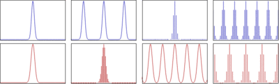
Spectral Leakage

Spectral leakage happens when the signal is not perfectly periodic within the DFT window. If a frequency component doesn't land exactly on a bin center, its energy spreads ("leaks") into neighboring bins, creating broad skirts instead of a sharp peak.

Why this happens:

1. The DFT implicitly assumes the signal repeats every $N$ samples
2. If the signal isn't periodic over that interval, the assumed repetition creates artificial discontinuities at the boundaries
3. These discontinuities act like a rectangular window multiplication, which has wide sidelobes in the frequency domain

Windowing reduces leakage by tapering the signal smoothly to zero at both ends before computing the DFT. Common window functions include:

• Hann: Good general-purpose choice, significant sidelobe reduction
• Hamming: Similar to Hann but with slightly different sidelobe behavior
• Blackman: Even lower sidelobes, but the main lobe is wider (worse resolution)

The trade-off with windowing is always the same: better sidelobe suppression comes at the cost of a wider main lobe, which reduces your effective frequency resolution.

DFT/FFT Applications

Filtering

Frequency-domain filtering follows a straightforward process:

1. Compute the DFT/FFT of the input signal
2. Modify the spectral coefficients $X[k]$ to suppress or retain desired frequencies
3. Compute the inverse DFT/FFT to get the filtered time-domain signal

Common filter types:

• Low-pass: Set $X[k] = 0$ for bins above a cutoff frequency, keeping only low-frequency content
• High-pass: Set $X[k] = 0$ for bins below a cutoff frequency, removing slow variations
• Band-pass: Retain only a specific frequency range, zeroing everything outside it
• Band-stop (notch): Remove a specific frequency range while keeping everything else

One thing to watch for: hard zeroing of coefficients can introduce ringing artifacts (Gibbs phenomenon) in the time domain. Gradual roll-offs tend to produce cleaner results.

Denoising

Denoising in the frequency domain works because signal and noise often occupy different spectral regions or have different amplitude characteristics.

The basic approach:

1. Compute the DFT/FFT of the noisy signal
2. Apply a threshold to the spectral coefficients
3. Inverse-transform to recover the cleaned signal

Two common thresholding strategies:

• Hard thresholding: Set any coefficient with magnitude below the threshold to zero; leave the rest unchanged
• Soft thresholding: Shrink all coefficients toward zero by the threshold amount, which produces smoother results

Choosing the right threshold involves balancing noise reduction against signal distortion. Too aggressive and you lose signal detail; too conservative and noise remains.

Feature Extraction

Spectral features extracted from the DFT/FFT are widely used for classification and analysis tasks. Some commonly computed features:

• Peak frequencies: The dominant frequency components (locations of magnitude peaks)
• Spectral centroid: The "center of mass" of the spectrum, often correlating with perceived brightness in audio
• Spectral bandwidth: How spread out the energy is around the centroid
• Spectral entropy: A measure of how uniform or concentrated the spectral energy distribution is (high entropy = noise-like; low entropy = tonal)

These features are used in applications like audio classification, speech recognition, vibration monitoring, and biomedical signal analysis. The DFT/FFT provides a compact, informative representation that's often much easier to work with than raw time-domain samples.