9.6 Multivariable calculus

Multivariable calculus expands single-variable calculus to functions with multiple inputs. It gives you the tools to analyze systems in higher dimensions, from fluid flow to economic models to machine learning algorithms. The concepts here build on each other: partial derivatives lead to gradients, gradients connect to optimization, and vector operations tie into the major theorems that unify the whole subject.

Functions of multiple variables

A function of multiple variables takes two or more inputs and produces an output. Where single-variable calculus deals with curves, multivariable calculus deals with surfaces, volumes, and higher-dimensional objects. This is the foundation for everything else in this unit.

Domain and range

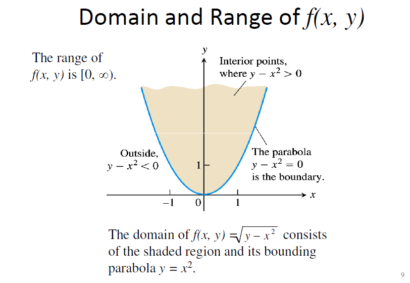
The domain of a multivariable function is the set of all valid input combinations. For a function $f(x, y)$, the domain is a region in the $xy$-plane. For $f(x, y, z)$, it's a region in 3D space.

• Restrictions on the domain come from the same rules as single-variable: no dividing by zero, no square roots of negative numbers, no logarithms of non-positive values
• The range is the set of all possible output values. Outputs can be scalar (a single number) or vector-valued (multiple components)
• Contour plots help visualize two-variable functions by drawing curves where the output is constant (think topographic maps showing elevation). Level surfaces do the same thing for three-variable functions.

Visualization techniques

• Contour plots draw curves of constant function value. Closely spaced contours mean the function is changing rapidly in that region.
• 3D surface plots graph $z = f(x, y)$ directly, revealing peaks, valleys, and saddle points
• Vector fields use arrows at each point to show magnitude and direction, useful for visualizing wind, force fields, or fluid flow
• Heat maps use color gradients to represent function values across a region (temperature distributions are a classic example)

Partial derivatives

A partial derivative measures how a function changes with respect to one variable while all other variables are held constant. The notation $\frac{\partial f}{\partial x}$ means "the rate of change of $f$ as $x$ changes, with everything else fixed."

To compute a partial derivative, treat every other variable as a constant and differentiate normally. For example, if $f(x, y) = x^2 y + 3y$, then $\frac{\partial f}{\partial x} = 2xy$ (treating $y$ as a constant).

• Geometrically, $\frac{\partial f}{\partial x}$ gives the slope of the surface in the $x$-direction at a point
• Higher-order partial derivatives involve differentiating again: $\frac{\partial^2 f}{\partial x \partial y}$ means you first differentiate with respect to $y$, then with respect to $x$
• Clairaut's theorem says that for most well-behaved functions, the order of mixed partials doesn't matter: $\frac{\partial^2 f}{\partial x \partial y} = \frac{\partial^2 f}{\partial y \partial x}$

Vector calculus

Vector calculus combines multivariable calculus with vector analysis. It provides the language for describing motion, forces, and fields in three-dimensional space, and it's the mathematical backbone of electromagnetism and fluid dynamics.

Vector fields

A vector field assigns a vector to every point in a region of space. Wind velocity at each point in the atmosphere is a vector field. So is the gravitational force field around a planet.

• Visualized using arrow plots, where each arrow shows the direction and magnitude of the vector at that point
• A conservative (or gradient) field can be written as the gradient of some scalar function, called a potential function. Gravity is conservative; friction is not.
• Two key operations on vector fields: divergence (a scalar measuring how much the field "spreads out") and curl (a vector measuring how much the field "rotates")

Line integrals

A line integral integrates a function along a curve or path rather than over an interval.

• Scalar line integrals add up a scalar quantity along a path (like finding the total mass of a wire with varying density)
• Vector line integrals compute quantities like the work done by a force field on an object moving along a path
• In a conservative field, the line integral depends only on the starting and ending points, not the path taken. This is called path independence.
• The fundamental theorem of line integrals says that for a gradient field $\vec{F} = \nabla f$, the line integral from point A to point B equals $f(B) - f(A)$

Surface integrals

Surface integrals extend double integrals to curved surfaces in 3D space.

• Scalar surface integrals compute things like the total mass of a curved sheet or the surface area itself
• Vector surface integrals (flux integrals) measure how much of a vector field passes through a surface
• Setting up a surface integral requires parameterizing the surface, which means expressing it in terms of two parameters
• Applications include calculating electric flux through a surface and fluid flow rates through membranes

Gradient and directional derivatives

The gradient and directional derivatives tell you how a multivariable function changes in any direction you choose. These are the core tools for optimization in multiple dimensions.

Gradient vector

The gradient of a scalar function $f(x, y, z)$ is the vector of all its partial derivatives:

$\nabla f = \left(\frac{\partial f}{\partial x}, \frac{\partial f}{\partial y}, \frac{\partial f}{\partial z}\right)$

• The gradient points in the direction of steepest increase of the function
• Its magnitude tells you the rate of change in that steepest direction
• The gradient is always perpendicular to level curves (in 2D) and level surfaces (in 3D). This is why contour lines on a map are perpendicular to the direction of steepest slope.

Directional derivatives

The directional derivative measures the rate of change of a function in any specified direction, not just along the coordinate axes.

• Calculated as the dot product of the gradient and a unit vector $\hat{u}$ in the desired direction: $D_{\hat{u}} f = \nabla f \cdot \hat{u}$
• Partial derivatives are special cases where $\hat{u}$ points along a coordinate axis
• The directional derivative is maximized when $\hat{u}$ points in the same direction as $\nabla f$, and minimized when it points opposite to $\nabla f$

Applications in optimization

• Gradient descent repeatedly steps in the direction of $-\nabla f$ to find local minima. This is the workhorse algorithm behind training neural networks.
• Critical points occur where $\nabla f = \vec{0}$. These are candidates for local maxima, local minima, or saddle points.
• The Hessian matrix (the matrix of all second partial derivatives) classifies critical points. Its determinant and eigenvalues tell you whether you're at a max, min, or saddle point.

Multiple integrals

Multiple integrals extend integration to functions of two or more variables. Where a single integral finds area under a curve, a double integral finds volume under a surface, and a triple integral accumulates a quantity over a 3D region.

Double integrals

A double integral $\iint f(x,y) \, dA$ integrates a function over a 2D region.

• Evaluated as iterated integrals: integrate with respect to one variable first, then the other
• The order of integration matters for difficulty. Sketching the region often reveals which order is simpler.
• Applications include computing volumes, areas of curved surfaces, centers of mass, and moments of inertia

Triple integrals

A triple integral $\iiint f(x,y,z) \, dV$ integrates over a 3D region.

• Evaluated as iterated integrals with three layers of integration (six possible orders)
• Choosing the right coordinate system can dramatically simplify the problem: use cylindrical coordinates for regions with circular symmetry and spherical coordinates for spherical regions
• Used to calculate volumes, masses of solid objects, and gravitational potentials

Change of variables

When a region has an awkward shape in Cartesian coordinates, a change of variables can simplify the integral.

1. Choose a new coordinate system that matches the geometry of the region (polar, cylindrical, spherical, or a custom transformation)
2. Express the integrand and the region boundaries in the new coordinates
3. Compute the Jacobian determinant, which accounts for how the transformation stretches or compresses area/volume
4. Multiply the integrand by the absolute value of the Jacobian and integrate

For example, switching to polar coordinates for a circular region replaces $dx \, dy$ with $r \, dr \, d\theta$, where $r$ is the Jacobian factor.

Divergence and curl

Divergence and curl are the two main differential operations on vector fields. They capture fundamentally different behaviors: divergence measures expansion/compression, and curl measures rotation.

Divergence of vector fields

The divergence of a vector field $\vec{F} = (F_1, F_2, F_3)$ is the scalar:

$\nabla \cdot \vec{F} = \frac{\partial F_1}{\partial x} + \frac{\partial F_2}{\partial y} + \frac{\partial F_3}{\partial z}$

• Positive divergence at a point means the field is acting as a source (spreading out)
• Negative divergence means it's acting as a sink (converging inward)
• Zero divergence everywhere means the field is incompressible (no net flow in or out)

Curl of vector fields

The curl of a vector field measures the tendency of the field to rotate around a point. It's computed as:

$\nabla \times \vec{F} = \left(\frac{\partial F_3}{\partial y} - \frac{\partial F_2}{\partial z},\; \frac{\partial F_1}{\partial z} - \frac{\partial F_3}{\partial x},\; \frac{\partial F_2}{\partial x} - \frac{\partial F_1}{\partial y}\right)$

• The curl is a vector: its direction is the axis of rotation, and its magnitude is the strength of rotation
• A field with zero curl everywhere is irrotational (conservative), meaning it can be written as the gradient of a scalar potential
• Non-zero curl indicates vorticity or circulation in the field

Physical interpretations

• In fluid dynamics, divergence represents expansion or compression of the fluid. Curl represents the local spinning of fluid particles.
• In electromagnetism, divergence of the electric field relates to charge density (Gauss's law). Divergence of the magnetic field is always zero (no magnetic monopoles).
• Faraday's law connects the curl of the electric field to a changing magnetic field. These relationships are encoded in Maxwell's equations.

Theorems in vector calculus

Three major theorems connect line, surface, and volume integrals. They're all generalizations of the fundamental theorem of calculus to higher dimensions, and they share a common structure: an integral over a region equals an integral over its boundary.

Green's theorem

Green's theorem relates a line integral around a closed curve in the plane to a double integral over the enclosed region.

$\oint_C (P \, dx + Q \, dy) = \iint_R \left(\frac{\partial Q}{\partial x} - \frac{\partial P}{\partial y}\right) dA$

• Converts between line integrals and area integrals in 2D
• Useful for computing areas: the area enclosed by a curve $C$ can be written as $\frac{1}{2} \oint_C (x \, dy - y \, dx)$
• Green's theorem is a special case of Stokes' theorem restricted to two dimensions

Stokes' theorem

Stokes' theorem generalizes Green's theorem to 3D. It relates the surface integral of the curl of a vector field to the line integral around the boundary of the surface.

$\iint_S (\nabla \times \vec{F}) \cdot d\vec{S} = \oint_C \vec{F} \cdot d\vec{r}$

• Connects the local rotation (curl) of a field over a surface to the global circulation around its boundary
• Used in electromagnetism to relate electric and magnetic fields
• The surface can be any surface bounded by the curve $C$, which gives you flexibility in choosing the easiest one to integrate over

Divergence theorem

The divergence theorem (Gauss's theorem) relates the flux of a vector field through a closed surface to the divergence inside the enclosed volume.

$\oiint_S \vec{F} \cdot d\vec{S} = \iiint_V (\nabla \cdot \vec{F}) \, dV$

• Converts between surface integrals and volume integrals
• Gauss's law in electrostatics is a direct application: the electric flux through a closed surface equals the enclosed charge divided by $\epsilon_0$
• Connects local behavior (divergence at each point) to global behavior (total flux through the boundary)

Optimization in multiple variables

Optimization in multivariable calculus finds the maximum or minimum values of functions with several inputs. The approach parallels single-variable optimization but requires more sophisticated tools.

Critical points

A critical point of $f(x, y)$ occurs where both $\frac{\partial f}{\partial x} = 0$ and $\frac{\partial f}{\partial y} = 0$ (or where a partial derivative is undefined).

To classify critical points, use the second derivative test with the Hessian:

1. Compute the Hessian determinant: $D = f_{xx} f_{yy} - (f_{xy})^2$

2. If $D > 0$ and $f_{xx} > 0$, the point is a local minimum

3. If $D > 0$ and $f_{xx} < 0$, the point is a local maximum

4. If $D < 0$, the point is a saddle point

5. If $D = 0$, the test is inconclusive

Constrained optimization

Often you need to optimize a function subject to constraints. For example, maximizing output given a fixed budget.

• For simple constraints, you can sometimes solve the constraint for one variable and substitute, reducing the problem to fewer variables
• For more complex constraints, Lagrange multipliers are the standard technique
• Inequality constraints (like $g(x,y) \leq c$) require the Karush-Kuhn-Tucker (KKT) conditions, which generalize Lagrange multipliers

Lagrange multipliers

The method of Lagrange multipliers finds extrema of $f(x, y)$ subject to the constraint $g(x, y) = c$.

1. Form the system of equations: $\nabla f = \lambda \nabla g$ and $g(x, y) = c$
2. This gives you a system with unknowns $x, y,$ and $\lambda$
3. Solve the system to find candidate points
4. Evaluate $f$ at each candidate to determine which gives the max or min

The geometric intuition: at the optimal point, the gradient of $f$ and the gradient of $g$ point in the same (or opposite) direction. The level curve of $f$ is tangent to the constraint curve.

Applications of multivariable calculus

Physics and engineering

• Electromagnetism: Maxwell's equations are written entirely in the language of vector calculus (divergence, curl, gradient)
• Fluid dynamics: the Navier-Stokes equations use multivariable calculus to describe flow patterns, pressure, and turbulence
• Thermodynamics: partial derivatives describe how state variables (pressure, volume, temperature) relate to each other
• Structural engineering: optimization techniques help design structures that minimize material use while meeting strength requirements

Economics and finance

• Utility functions with multiple goods use partial derivatives to analyze marginal utility and consumer choice
• Production functions like the Cobb-Douglas model $Q = A L^\alpha K^\beta$ use multivariable calculus to study how labor and capital affect output
• Portfolio optimization applies constrained optimization to balance risk and return across multiple assets
• Econometrics relies on multivariable calculus for regression analysis and maximum likelihood estimation

Computer graphics

• 3D surface modeling uses parametric equations and multivariable functions to represent shapes and textures
• Ray tracing algorithms use vector calculus to compute light paths and surface intersections
• Shading calculations depend on normal vectors and directional derivatives to simulate how light interacts with surfaces

Differential equations

Differential equations involving multiple variables are called partial differential equations (PDEs). They model systems where quantities depend on more than one independent variable, like position and time.

Partial differential equations

• A PDE involves partial derivatives of an unknown function with respect to two or more variables
• PDEs are classified as elliptic (steady-state problems, like Laplace's equation), parabolic (diffusion processes, like the heat equation), or hyperbolic (wave propagation, like the wave equation)
• Solution methods include separation of variables, Fourier series, and numerical techniques
• Applications span quantum mechanics, fluid dynamics, and financial modeling (the Black-Scholes equation for option pricing is a PDE)

Systems of differential equations

• Multiple coupled differential equations describe systems where several quantities influence each other simultaneously
• Linear systems can be solved using matrix methods and eigenvalue analysis
• Nonlinear systems typically require numerical methods or qualitative analysis techniques
• Phase plane analysis provides geometric insight by plotting trajectories in the space of dependent variables
• Classic examples include predator-prey models in ecology and coupled oscillators in physics

Numerical methods

When exact solutions aren't available, numerical methods approximate solutions on a discrete grid.

• Finite difference methods replace derivatives with difference quotients on a grid
• Runge-Kutta methods provide accurate step-by-step solutions for initial value problems (the fourth-order version is widely used)
• Finite element methods break complex domains into small elements, making them well-suited for irregular geometries
• Spectral methods use global basis functions (like Fourier modes) for high accuracy on smooth problems

Manifolds and surfaces

Manifolds and surfaces extend the study of curves to higher-dimensional objects. This is where multivariable calculus connects to differential geometry.

Parameterization of surfaces

A parameterization describes a surface using two parameters, typically $u$ and $v$. The surface is given by a vector-valued function $\vec{r}(u, v) = (x(u,v), \, y(u,v), \, z(u,v))$.

• Standard examples: a sphere can be parameterized using angles $\theta$ and $\phi$; a cylinder using angle $\theta$ and height $z$
• Parameterization is required for computing surface integrals, surface area, and normal vectors
• Surfaces defined implicitly by an equation like $F(x, y, z) = 0$ can often be converted to parametric form

Tangent planes

The tangent plane at a point on a surface is the best flat approximation to the surface at that point.

• For a surface $z = f(x, y)$, the tangent plane at $(a, b, f(a,b))$ is: $z = f(a,b) + f_x(a,b)(x - a) + f_y(a,b)(y - b)$
• The normal vector to the tangent plane is perpendicular to the surface at that point
• Tangent planes are used in linear approximation, optimization on surfaces, and computing surface normals for lighting in computer graphics

Curvature and normal vectors

Curvature quantifies how much a surface bends at each point.

• Principal curvatures $\kappa_1$ and $\kappa_2$ are the maximum and minimum curvatures at a point, measured in perpendicular directions
• Gaussian curvature $K = \kappa_1 \kappa_2$ classifies the local shape: positive (bowl-like), zero (flat or cylindrical), or negative (saddle-like)
• Mean curvature $H = \frac{\kappa_1 + \kappa_2}{2}$ appears in minimal surface problems (soap films minimize mean curvature)
• These concepts are foundational in differential geometry, general relativity, and computer-aided design