6.4 Probability distributions

Probability distributions give you a framework for understanding and predicting random events. They're the backbone of statistical analysis, connecting raw randomness to patterns you can actually work with for predictions and decision-making.

This guide covers discrete and continuous distributions, their key properties (mean, variance, skewness), joint distributions, sampling distributions, and how all of this gets applied in fields like finance, engineering, and data science.

Fundamentals of probability distributions

Probability distributions describe how likely different outcomes are for a random process. Once you understand the type of distribution you're dealing with, you can calculate probabilities, make predictions, and compare different scenarios mathematically.

Concept of random variables

A random variable assigns a numerical value to each outcome of a random process. There are two types:

• Discrete random variables take on distinct, countable values. Think: the number of heads in 10 coin flips. Their probabilities are described by a probability mass function (PMF), which gives the exact probability of each specific outcome.
• Continuous random variables can take any value within a range. Think: the height of a randomly selected person. Their probabilities are described by a probability density function (PDF), which gives the relative likelihood across a continuum of values.

Types of probability distributions

• Discrete distributions deal with countable outcomes (binomial, Poisson)
• Continuous distributions handle outcomes that can be any value in a range (normal, exponential)
• Univariate distributions involve a single random variable
• Multivariate distributions describe relationships between two or more random variables
• Empirical distributions are derived from observed data rather than theoretical models

Probability density functions

A PDF is a mathematical function that describes the likelihood of different outcomes for a continuous random variable. You don't read probabilities directly off the curve. Instead, the area under the curve over an interval gives you the probability of the variable falling in that range.

• The function must be non-negative for all possible values
• The total area under the curve always equals 1 (total probability)
• The shape of the PDF reveals characteristics like symmetry and spread

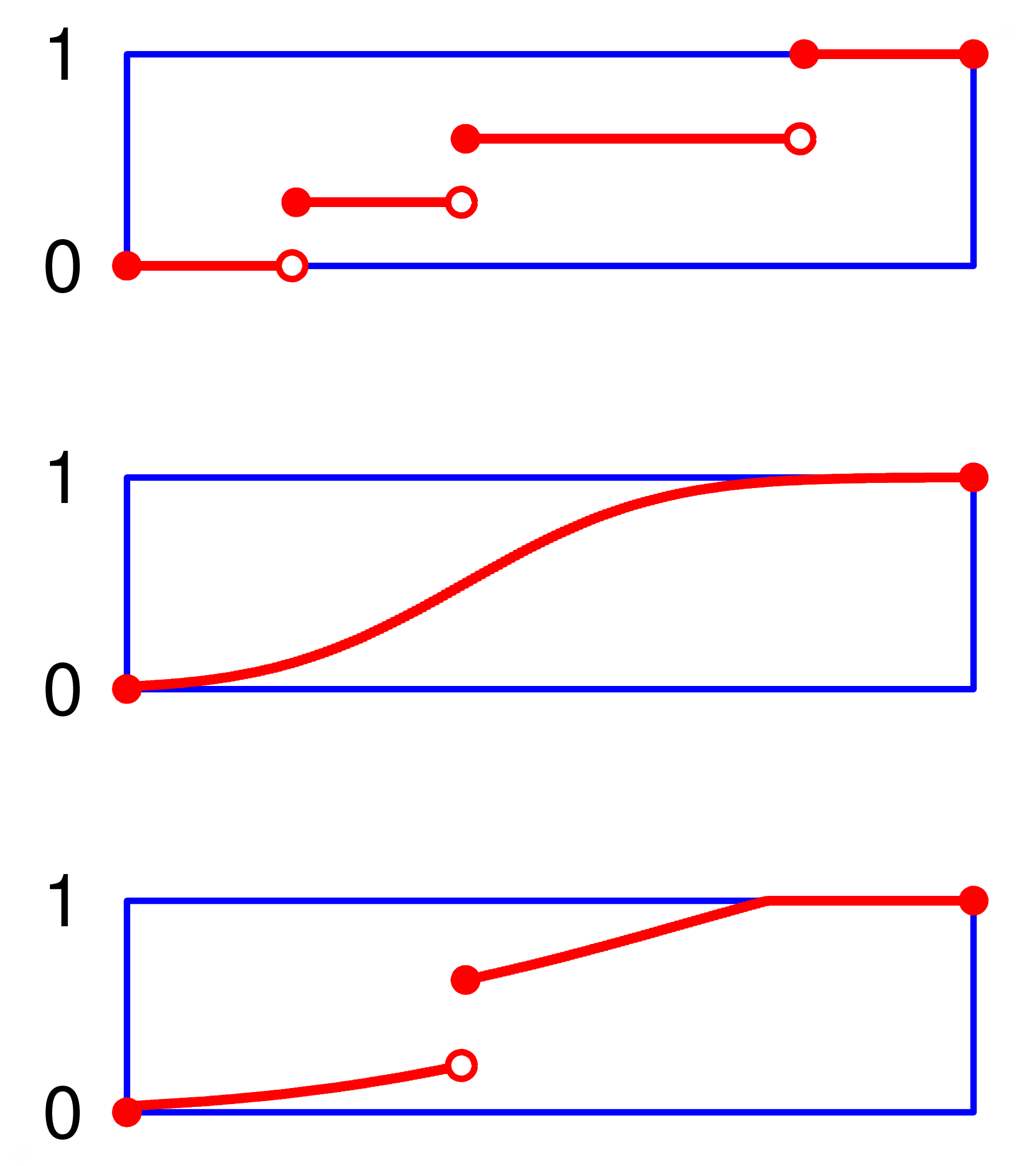
Cumulative distribution functions

A cumulative distribution function (CDF) gives the probability that a random variable takes a value less than or equal to a given point. It answers the question: what's the probability of getting this value or lower?

• For discrete distributions, you calculate it by summing probabilities of all values up to that point
• For continuous distributions, you integrate the PDF up to that point
• The CDF is always monotonically increasing, ranging from 0 to 1
• CDFs are especially useful for calculating probabilities over ranges and finding percentiles

Discrete probability distributions

Discrete distributions model situations where outcomes are countable. Each distribution below fits a specific type of scenario, so recognizing which one applies is half the battle.

Bernoulli distribution

The simplest discrete distribution. It models a single trial with exactly two outcomes: success (1) or failure (0).

• PMF: $P(X=x) = p^x(1-p)^{1-x}$ where $x$ is 0 or 1
• Mean: $E(X) = p$
• Variance: $Var(X) = p(1-p)$

A coin flip is the classic example. Any yes/no question or single pass/fail event follows a Bernoulli distribution.

Binomial distribution

This extends the Bernoulli to multiple trials. It models the number of successes in $n$ independent trials, each with the same probability $p$ of success.

• PMF: $P(X=k) = \binom{n}{k}p^k(1-p)^{n-k}$
• Mean: $E(X) = np$
• Variance: $Var(X) = np(1-p)$

For example, if a factory produces items with a 3% defect rate and you inspect 50 items, the number of defective items follows a binomial distribution with $n=50$ and $p=0.03$.

Poisson distribution

Models the number of events occurring in a fixed interval of time or space, where events happen independently at a constant average rate.

• PMF: $P(X=k) = \frac{\lambda^k e^{-\lambda}}{k!}$
• Both the mean and variance equal $\lambda$ (the rate parameter)
• Approximates the binomial distribution when $n$ is large and $p$ is small

A hospital emergency room that averages 4.2 arrivals per hour would use a Poisson distribution with $\lambda = 4.2$ to model the number of arrivals in any given hour.

Geometric distribution

Models how many trials you need before getting your first success in a sequence of independent Bernoulli trials.

• PMF: $P(X=k) = (1-p)^{k-1}p$
• Mean: $E(X) = \frac{1}{p}$
• Variance: $Var(X) = \frac{1-p}{p^2}$

If you're rolling a die waiting for a six, the number of rolls needed follows a geometric distribution with $p = \frac{1}{6}$, giving an expected value of 6 rolls.

Continuous probability distributions

Continuous distributions model variables that can take any value in a range. Because there are infinitely many possible values, the probability of any single exact value is technically zero. You always work with probabilities over intervals.

Uniform distribution

The simplest continuous distribution: all outcomes in a range $[a, b]$ are equally likely.

• PDF: $f(x) = \frac{1}{b-a}$ for $a \leq x \leq b$
• Mean: $E(X) = \frac{a+b}{2}$
• Variance: $Var(X) = \frac{(b-a)^2}{12}$

Random number generators typically produce values from a uniform distribution. If a bus arrives at a stop every 15 minutes and you show up at a random time, your wait time follows a uniform distribution on $[0, 15]$.

Normal distribution

The famous bell curve. It shows up constantly in nature and statistics because of the Central Limit Theorem.

• PDF: $f(x) = \frac{1}{\sigma\sqrt{2\pi}}e^{-\frac{(x-\mu)^2}{2\sigma^2}}$
• Fully characterized by its mean ($\mu$) and standard deviation ($\sigma$)
• Symmetric around the mean
• The 68-95-99.7 rule: approximately 68% of data falls within 1 standard deviation of the mean, 95% within 2, and 99.7% within 3
• The Central Limit Theorem states that the distribution of sample means approaches a normal distribution as sample size increases, regardless of the population's shape

Applications include modeling human heights, IQ scores, and measurement errors in experiments.

Exponential distribution

Models the time between consecutive events in a Poisson process.

• PDF: $f(x) = \lambda e^{-\lambda x}$ for $x \geq 0$
• Mean: $E(X) = \frac{1}{\lambda}$
• Variance: $Var(X) = \frac{1}{\lambda^2}$
• Has the memoryless property: the probability of waiting another 5 minutes is the same whether you've already waited 2 minutes or 20 minutes

If customers arrive at a store at an average rate of 3 per hour, the time between arrivals follows an exponential distribution with $\lambda = 3$, giving a mean wait of $\frac{1}{3}$ hour (20 minutes).

Gamma distribution

Generalizes the exponential distribution. While the exponential models the time until one event, the gamma models the time until $\alpha$ events occur.

• PDF: $f(x) = \frac{\beta^\alpha}{\Gamma(\alpha)}x^{\alpha-1}e^{-\beta x}$ for $x > 0$
• Shape parameter ($\alpha$) and rate parameter ($\beta$) determine the distribution's behavior
• Mean: $E(X) = \frac{\alpha}{\beta}$
• Variance: $Var(X) = \frac{\alpha}{\beta^2}$
• When $\alpha = 1$, the gamma distribution reduces to the exponential distribution

Used in modeling rainfall amounts, insurance claim sizes, and total service times in queuing systems.

Properties of distributions

These properties give you standardized ways to describe and compare any distribution. Knowing the mean and variance of a distribution tells you a lot, but skewness and kurtosis fill in the rest of the picture.

Expected value

The expected value (mean) represents the long-run average outcome of a random variable. It's the value you'd converge on if you repeated the experiment infinitely many times.

• For discrete distributions: $E(X) = \sum_{i} x_i P(X=x_i)$
• For continuous distributions: $E(X) = \int_{-\infty}^{\infty} x f(x) dx$

The expected value provides a measure of central tendency and is widely used in decision-making and risk assessment. For example, the expected return on an investment helps you compare options.

Variance and standard deviation

Variance measures how spread out a distribution is around its mean. A small variance means values cluster tightly; a large variance means they're more dispersed.

• For discrete distributions: $Var(X) = \sum_{i} (x_i-\mu)^2 P(X=x_i)$
• For continuous distributions: $Var(X) = \int_{-\infty}^{\infty} (x-\mu)^2 f(x) dx$

Standard deviation is the square root of variance. It's often more useful in practice because it's in the same units as the original data, making it easier to interpret.

Skewness and kurtosis

Skewness measures asymmetry in a distribution:

• Positive skew (right-skewed): longer tail on the right, bulk of data on the left. Income distributions are a classic example.
• Negative skew (left-skewed): longer tail on the left.
• A perfectly symmetric distribution (like the normal) has skewness of 0.

Kurtosis measures how heavy the tails are:

• Leptokurtic (kurtosis > 3): heavier tails and a sharper peak than normal. More extreme outliers.
• Platykurtic (kurtosis < 3): lighter tails and a flatter peak.
• Mesokurtic (kurtosis = 3): the normal distribution is the baseline.

Both are used in financial modeling to assess risk beyond what variance alone can capture.

Moments of distributions

Moments provide a systematic way to describe a distribution's shape. Each moment captures a different aspect:

• First moment: mean (location)
• Second central moment: variance (spread)
• Third central moment: related to skewness (asymmetry)
• Fourth central moment: related to kurtosis (tail weight)

Moment generating functions (MGFs) uniquely determine a probability distribution. If two distributions have the same MGF, they're the same distribution. MGFs also simplify calculations when working with sums of independent random variables.

Joint probability distributions

When you're dealing with two or more random variables at once, joint distributions let you analyze how they behave together, not just individually.

Bivariate distributions

A bivariate distribution describes the joint behavior of two random variables. For discrete variables, you use a joint PMF; for continuous variables, a joint PDF.

• These allow you to calculate probabilities for events involving both variables simultaneously
• Visualized using 3D surface plots or contour plots for continuous cases
• Used for analyzing relationships like height and weight, or pairs of stock prices

Marginal distributions

A marginal distribution extracts the distribution of one variable from a joint distribution, ignoring the other variable entirely.

• For discrete variables: $P(X=x) = \sum_y P(X=x, Y=y)$
• For continuous variables: $f_X(x) = \int_{-\infty}^{\infty} f_{X,Y}(x,y) \, dy$

You "marginalize out" the variable you don't care about by summing (discrete) or integrating (continuous) over all its possible values.

Conditional distributions

A conditional distribution describes the probability distribution of one variable given that the other variable takes a specific value.

• For discrete variables: $P(Y=y|X=x) = \frac{P(X=x, Y=y)}{P(X=x)}$
• For continuous variables: $f_{Y|X}(y|x) = \frac{f_{X,Y}(x,y)}{f_X(x)}$

This is the foundation of Bayesian inference, where you update your beliefs about one variable after observing another.

Covariance and correlation

Covariance measures how two random variables move together:

$Cov(X,Y) = E[(X-\mu_X)(Y-\mu_Y)]$

• Positive covariance: variables tend to increase together
• Negative covariance: when one increases, the other tends to decrease
• Zero covariance: no linear relationship (but there could still be a non-linear one)

The correlation coefficient normalizes covariance to a $-1$ to $1$ scale, making it easier to interpret:

$\rho_{X,Y} = \frac{Cov(X,Y)}{\sigma_X \sigma_Y}$

A correlation of $+1$ means perfect positive linear relationship; $-1$ means perfect negative; $0$ means no linear relationship.

Sampling distributions

A sampling distribution describes how a sample statistic (like the sample mean) varies across all possible samples of a given size from a population. This is what makes statistical inference possible.

Central limit theorem

The Central Limit Theorem (CLT) is one of the most important results in statistics. It states that the distribution of sample means approaches a normal distribution as sample size increases, regardless of the population's original shape (as long as the population has finite variance).

• A sample size of at least 30 is the common rule of thumb for the CLT to kick in
• The mean of the sampling distribution equals the population mean
• The standard error decreases as sample size increases, meaning larger samples give more precise estimates

This is why the normal distribution appears so often in statistical methods.

Distribution of sample mean

For a sample of size $n$ drawn from a population with mean $\mu$ and standard deviation $\sigma$:

• The sampling distribution of $\bar{X}$ has mean $\mu$
• The standard error is: $SE_{\bar{X}} = \frac{\sigma}{\sqrt{n}}$
• For large $n$, this distribution is approximately normal (by the CLT)

This is what you use when constructing confidence intervals or performing hypothesis tests about population means.

Distribution of sample variance

For samples drawn from a normally distributed population:

• The quantity $\frac{(n-1)S^2}{\sigma^2}$ follows a chi-square distribution with $n-1$ degrees of freedom
• Mean of the sampling distribution: $E(S^2) = \sigma^2$ (the sample variance is an unbiased estimator)
• Variance of the sampling distribution: $Var(S^2) = \frac{2\sigma^4}{n-1}$

This result is used in hypothesis tests and confidence intervals for population variance.

Chi-square distribution

The chi-square distribution arises from summing the squares of independent standard normal random variables. It's characterized by its degrees of freedom (df).

• Mean = df
• Variance = 2 × df
• Right-skewed, but becomes more symmetric as df increases
• Used in goodness-of-fit tests, tests of independence for categorical data, and variance-related inference

Applications of probability distributions

Statistical inference

Statistical inference uses probability distributions to draw conclusions about populations from sample data. The core activities are:

• Estimation: finding point estimates and confidence intervals for population parameters
• Hypothesis testing: making formal decisions about population characteristics
• Bayesian inference: updating probability estimates as new evidence arrives

Sampling distributions quantify the uncertainty in your estimates, which is what separates statistical reasoning from guessing.

Hypothesis testing

Hypothesis testing is a formal procedure for deciding whether sample data provides enough evidence to reject a claim about a population.

1. State the null hypothesis ($H_0$): the default assumption (e.g., no effect, no difference)
2. State the alternative hypothesis ($H_1$): the claim you're testing
3. Calculate a test statistic from the sample data. Under $H_0$, this statistic follows a known distribution
4. Find the p-value: the probability of getting results as extreme as (or more extreme than) what you observed, assuming $H_0$ is true
5. Compare the p-value to your significance level ($\alpha$, typically 0.05). If the p-value is less than $\alpha$, reject $H_0$

Applications include testing whether a new drug is more effective than a placebo, or whether two manufacturing processes produce different defect rates.

Confidence intervals

A confidence interval provides a range of plausible values for a population parameter, along with a specified confidence level (commonly 95%).

• For a population mean (small sample): $\bar{X} \pm t_{\alpha/2, \, n-1} \frac{s}{\sqrt{n}}$
• For a population proportion: $\hat{p} \pm z_{\alpha/2} \sqrt{\frac{\hat{p}(1-\hat{p})}{n}}$

The width of the interval depends on three things: the confidence level, the sample size, and the variability in the data. Larger samples and lower confidence levels produce narrower intervals.

Risk assessment and decision making

• Expected value and variance guide risk-reward tradeoffs
• Value at Risk (VaR) uses distribution tails to quantify potential losses at a given confidence level
• Monte Carlo simulations generate thousands of random outcomes based on specified distributions to model complex scenarios
• Decision trees incorporate probabilities of different outcomes to evaluate choices

Applications span financial portfolio management, insurance pricing, and project planning.

Transformations of random variables

Transformations let you derive new distributions from existing ones. If you know the distribution of $X$, you can often figure out the distribution of $Y = g(X)$.

Linear transformations

A linear transformation takes the form $Y = aX + b$. The effects on the distribution are predictable:

• Mean: $E(Y) = aE(X) + b$
• Variance: $Var(Y) = a^2 Var(X)$

The shape of the distribution stays the same; only the location and scale change. Converting temperatures from Celsius to Fahrenheit ($F = 1.8C + 32$) is a linear transformation. Standardization ($Z = \frac{X - \mu}{\sigma}$) is another common example, converting any distribution to one with mean 0 and standard deviation 1.

Non-linear transformations

Non-linear transformations like $Y = X^2$ or $Y = \ln(X)$ change the shape of the distribution, not just its location and scale.

For continuous distributions, you use the change of variable technique:

1. Express $x$ in terms of $y$: find the inverse function $x = g^{-1}(y)$
2. Compute the Jacobian (the derivative $\frac{dx}{dy}$), which accounts for how the transformation stretches or compresses probability
3. The new PDF is: $f_Y(y) = f_X(g^{-1}(y)) \cdot \left|\frac{dx}{dy}\right|$

Logarithmic transformations are commonly used to convert right-skewed data (like income) into something closer to a normal distribution.

Convolution of distributions

Convolution gives you the distribution of the sum of independent random variables.

• For discrete variables: the PMF of the sum is the convolution of the individual PMFs
• For continuous variables: the PDF of the sum is the convolution of the individual PDFs
• The convolution theorem states that the Fourier transform of a convolution equals the product of the individual Fourier transforms, which often simplifies computation

This comes up when modeling total waiting times, aggregate insurance claims, or combined signals in engineering.

Moment generating functions

The moment generating function (MGF) of a random variable $X$ is defined as:

$M_X(t) = E[e^{tX}]$

Why MGFs are useful:

• They uniquely determine a distribution. Same MGF = same distribution.
• You can find the $n$th moment by taking the $n$th derivative of $M_X(t)$ and evaluating at $t = 0$
• For sums of independent random variables, the MGF of the sum equals the product of the individual MGFs, which is much simpler than convolution

Probability distributions in real-world

Financial modeling

• Normal distribution: models short-term stock returns
• Log-normal distribution: models asset prices over time (prices can't go negative, and returns compound)
• Student's t-distribution: captures the heavier tails observed in financial returns compared to the normal
• Poisson distribution: models rare events like defaults or market crashes
• Copulas: model dependencies between multiple financial variables
• VaR calculations rely on distribution tails to estimate worst-case losses at a given confidence level

Quality control

• Binomial distribution: models defective items in a sample (e.g., 3 defectives out of 100 inspected)
• Poisson distribution: models rare defects in large production runs
• Normal distribution: describes variation in continuous measurements (part dimensions, fill weights)
• Exponential distribution: models time between failures
• Weibull distribution: characterizes product lifetimes with varying failure rates over time
• Control charts use these distributions to set limits and flag when a process drifts out of specification

Reliability engineering

• Exponential distribution: models constant failure rates (common for electronics)
• Weibull distribution: handles failure rates that change over a product's lifetime (increasing wear-out, or decreasing infant mortality)
• Gamma distribution: models cumulative damage or wear-out processes
• Log-normal distribution: represents repair times or time-to-failure for certain systems
• Extreme value distributions: model maximum loads or stresses on structures
• Reliability functions derived from these distributions help predict maintenance schedules and design redundant systems

Data science applications

• Normal distribution: underlies many classical statistical techniques (regression, ANOVA)
• Poisson distribution: models count data in large datasets (click-through rates, fraud occurrences)
• Exponential and Pareto distributions: describe heavy-tailed phenomena in network science and web traffic
• Multinomial distribution: models categorical outcomes in classification tasks
• Beta distribution: represents probabilities or proportions in Bayesian inference
• Dirichlet distribution: generalizes the beta distribution for modeling distributions over multiple categories (used in topic modeling)