9.1 Limits

Definition of limits

Limits describe how a function behaves as its input gets closer and closer to a specific value. They're the core idea underlying all of calculus: derivatives, integrals, and continuity all depend on limits.

Intuitive understanding

A limit asks: what value does $f(x)$ approach as $x$ gets closer to some target? The function doesn't need to actually equal that value at the target point. It might not even be defined there. What matters is the trend.

• Graphically, you're looking at the y-value the curve settles toward as x moves toward a particular spot.
• This is especially useful near points where the function has holes, jumps, or vertical asymptotes.

For example, $f(x) = \frac{x^2 - 1}{x - 1}$ is undefined at $x = 1$, but as $x$ approaches 1, the function approaches 2. So $\lim_{x \to 1} f(x) = 2$.

Formal epsilon-delta definition

The formal definition makes the intuitive idea precise using two quantities: $\varepsilon$ (epsilon) and $\delta$ (delta).

$\lim_{x \to a} f(x) = L$ means: for every $\varepsilon > 0$, there exists a $\delta > 0$ such that whenever $0 < |x - a| < \delta$, we have $|f(x) - L| < \varepsilon$.

In plain terms: no matter how tight a tolerance ($\varepsilon$) you set around the output $L$, you can always find a small enough window ($\delta$) around the input $a$ that keeps all outputs within that tolerance. This definition provides the rigorous foundation for proving limit properties and theorems.

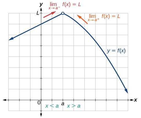
One-sided vs two-sided limits

Sometimes a function behaves differently depending on which direction you approach from.

• Left-hand limit $\lim_{x \to a^-} f(x)$: only considers values of $x$ less than $a$ (approaching from the left).
• Right-hand limit $\lim_{x \to a^+} f(x)$: only considers values of $x$ greater than $a$ (approaching from the right).
• Two-sided limit $\lim_{x \to a} f(x)$ exists only when both one-sided limits exist and are equal.

One-sided limits are particularly useful at endpoints of a function's domain and at jump discontinuities, where the left and right behaviors differ.

Evaluating limits

Several techniques exist for computing limits. The right method depends on the form of the function and what happens when you try the simplest approach first.

Direct substitution method

Always try this first. If the function is continuous at the point you care about, just plug in the value.

For example: $\lim_{x \to 3} (2x + 1) = 2(3) + 1 = 7$.

This works for polynomials, most rational functions (where the denominator isn't zero), and standard transcendental functions like $\sin x$ and $e^x$. When substitution gives you a well-defined number, you're done. When it produces something like $\frac{0}{0}$, you need a different technique.

Factoring techniques

When direct substitution yields $\frac{0}{0}$, the numerator and denominator likely share a common factor. Factor both, cancel the shared term, then try substitution again.

Example: $\lim_{x \to 2} \frac{x^2 - 4}{x - 2}$

1. Direct substitution gives $\frac{0}{0}$.

2. Factor the numerator: $x^2 - 4 = (x-2)(x+2)$.

3. Cancel: $\frac{(x-2)(x+2)}{x-2} = x+2$ (for $x \neq 2$).

4. Substitute: $2 + 2 = 4$.

This process also reveals removable discontinuities: the original function has a hole at $x = 2$, but the limit still equals 4.

Rationalization strategy

When the expression involves square roots (or other radicals), multiply the numerator and denominator by the conjugate to eliminate the radical.

Example: $\lim_{x \to 0} \frac{\sqrt{x+4} - 2}{x}$

1. Direct substitution gives $\frac{0}{0}$.

2. Multiply by the conjugate: $\frac{\sqrt{x+4} - 2}{x} \cdot \frac{\sqrt{x+4} + 2}{\sqrt{x+4} + 2}$.

3. The numerator becomes $(x+4) - 4 = x$.

4. Simplify: $\frac{x}{x(\sqrt{x+4}+2)} = \frac{1}{\sqrt{x+4}+2}$.

5. Substitute $x = 0$: $\frac{1}{\sqrt{4}+2} = \frac{1}{4}$.

L'Hôpital's rule

This is a powerful tool for indeterminate forms $\frac{0}{0}$ or $\frac{\infty}{\infty}$. If $\lim_{x \to a} f(x)$ and $\lim_{x \to a} g(x)$ are both 0 or both $\pm\infty$, then:

$\lim_{x \to a} \frac{f(x)}{g(x)} = \lim_{x \to a} \frac{f'(x)}{g'(x)}$

provided the right-hand limit exists. You can apply the rule repeatedly if the result is still indeterminate. Just make sure you verify the indeterminate form each time before reapplying.

Types of limits

Finite limits

A finite limit means the function approaches a specific real number. Written as $\lim_{x \to a} f(x) = L$, where $L$ is finite. This is the most common type and often indicates the function is well-behaved near that point, even if it's not defined exactly at $a$.

Infinite limits

An infinite limit means the function's output grows without bound as $x$ approaches some value. For instance, $\lim_{x \to 0} \frac{1}{x^2} = \infty$.

• $\lim_{x \to a} f(x) = \infty$ means the function increases without bound.
• $\lim_{x \to a} f(x) = -\infty$ means it decreases without bound.

Infinite limits signal vertical asymptotes on the graph. Technically, when we say a limit "equals infinity," the limit doesn't exist as a real number; the notation describes the specific way it fails to exist.

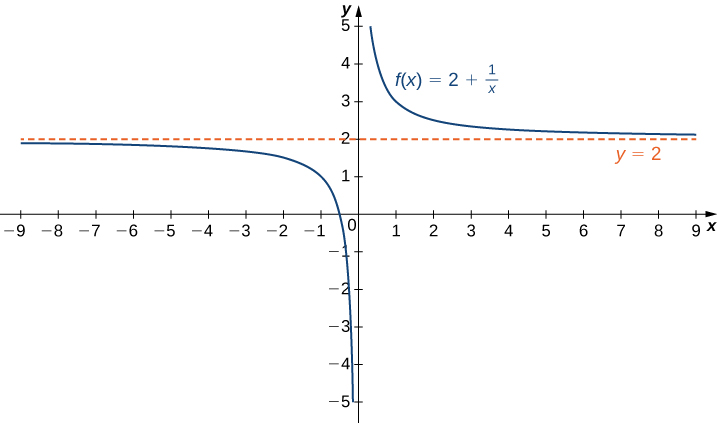
Limits at infinity

These describe what happens to $f(x)$ as $x$ itself grows very large (positive or negative).

• $\lim_{x \to \infty} \frac{1}{x} = 0$: the function flattens toward zero.
• $\lim_{x \to \infty} \frac{3x^2 + 1}{x^2 - 5} = 3$: compare leading terms to find horizontal asymptotes.

Limits at infinity reveal horizontal asymptotes and the long-term behavior of a function. For rational functions, compare the degrees of the numerator and denominator: same degree gives the ratio of leading coefficients, higher degree on top means the limit is infinite, and higher degree on the bottom means the limit is zero.

Limit properties

These properties let you break complicated limits into simpler pieces, provided each individual limit exists.

Sum and difference rules

$\lim_{x \to a} [f(x) \pm g(x)] = \lim_{x \to a} f(x) \pm \lim_{x \to a} g(x)$

You can evaluate the limit of a sum (or difference) by taking the limits separately and combining. This works as long as both individual limits exist and are finite.

Product and quotient rules

• Product: $\lim_{x \to a} [f(x) \cdot g(x)] = \lim_{x \to a} f(x) \cdot \lim_{x \to a} g(x)$
• Quotient: $\lim_{x \to a} \frac{f(x)}{g(x)} = \frac{\lim_{x \to a} f(x)}{\lim_{x \to a} g(x)}$, provided $\lim_{x \to a} g(x) \neq 0$

When the denominator's limit is zero, the quotient rule doesn't apply directly, and you'll need techniques like factoring, rationalization, or L'Hôpital's rule.

Composition of functions

For a composite function $f(g(x))$: if $\lim_{x \to a} g(x) = L$ and $f$ is continuous at $L$, then:

$\lim_{x \to a} f(g(x)) = f\left(\lim_{x \to a} g(x)\right) = f(L)$

The continuity requirement on the outer function $f$ is essential here. This property also provides the conceptual basis for the chain rule in differentiation.

Continuity and limits

Continuity ties together the limit of a function and its actual value. A continuous function is one where limits behave exactly as you'd hope.

Definition of continuity

A function $f(x)$ is continuous at a point $a$ if all three conditions hold:

1. $f(a)$ is defined.
2. $\lim_{x \to a} f(x)$ exists.
3. $\lim_{x \to a} f(x) = f(a)$.

If any condition fails, the function is discontinuous at $a$. For continuous functions, evaluating a limit is the same as plugging in the value, which is why direct substitution works on them.

Continuity underpins major theorems like the Intermediate Value Theorem and the Extreme Value Theorem.

Types of discontinuities

• Jump discontinuity: Both one-sided limits exist but aren't equal. The graph has a visible "jump" (e.g., piecewise functions like the floor function).
• Removable discontinuity: The limit exists, but either $f(a)$ is undefined or $f(a) \neq \lim_{x \to a} f(x)$. The graph has a "hole" that could be filled by redefining the function at that point.
• Infinite discontinuity: The function approaches $\pm\infty$ near the point, creating a vertical asymptote (e.g., $\frac{1}{x}$ at $x = 0$).
• Oscillating discontinuity: The function oscillates infinitely without settling on a value (e.g., $\sin\left(\frac{1}{x}\right)$ as $x \to 0$).

Intermediate value theorem

If $f(x)$ is continuous on the closed interval $[a, b]$, and $k$ is any value between $f(a)$ and $f(b)$, then there exists at least one $c$ in $[a, b]$ such that $f(c) = k$.

Intuitively, a continuous function can't skip over values. If $f(1) = -3$ and $f(5) = 7$, then somewhere between 1 and 5, the function must equal zero (and every other value between $-3$ and $7$). This theorem is the basis for root-finding methods like the bisection algorithm.

Applications of limits

Rates of change

The derivative, which measures instantaneous rate of change, is defined as a limit:

$f'(x) = \lim_{h \to 0} \frac{f(x+h) - f(x)}{h}$

This takes the average rate of change over a shrinking interval and finds what it approaches as the interval width goes to zero. Applications include velocity in physics (derivative of position), marginal cost in economics (derivative of total cost), and optimization across engineering and finance.

Tangent lines

The slope of the tangent line to $y = f(x)$ at the point $(a, f(a))$ is exactly $f'(a)$, which comes from the same limit definition above. The tangent line equation is:

$y - f(a) = f'(a)(x - a)$

Tangent lines give the best linear approximation of a function near a point. This idea is used in linear approximation, Newton's method for root-finding, and computer graphics for rendering smooth curves.

Area under curves

Limits also define the definite integral. You approximate the area under $f(x)$ from $a$ to $b$ using $n$ rectangles (a Riemann sum), then take the limit as $n \to \infty$:

$\int_a^b f(x)\,dx = \lim_{n \to \infty} \sum_{i=1}^n f(x_i)\Delta x$

As the rectangles get thinner, the approximation gets better, and the limit gives the exact area. This connects to calculating work done by a variable force, probabilities for continuous distributions, and accumulated quantities in general.

Common limit forms

Indeterminate forms

When direct substitution produces an expression whose value can't be determined without further work, you have an indeterminate form. The seven standard indeterminate forms are:

$\frac{0}{0}, \quad \frac{\infty}{\infty}, \quad 0 \cdot \infty, \quad \infty - \infty, \quad 0^0, \quad 1^\infty, \quad \infty^0$

These are "indeterminate" because expressions with these forms can converge to different values depending on the specific functions involved. Each requires algebraic manipulation, L'Hôpital's rule, or logarithmic techniques to resolve.

Trigonometric limits

Several standard trig limits appear frequently and are worth memorizing:

• $\lim_{x \to 0} \frac{\sin x}{x} = 1$
• $\lim_{x \to 0} \frac{\tan x}{x} = 1$
• $\lim_{x \to 0} \frac{1 - \cos x}{x} = 0$

The first one, $\frac{\sin x}{x} \to 1$, is foundational. It's typically proved using the Squeeze Theorem and a geometric argument with the unit circle. Many other trig limits can be derived from it.

Exponential and logarithmic limits

Two key limits define the behavior of exponential and logarithmic functions:

• $\lim_{x \to \infty} \left(1 + \frac{1}{x}\right)^x = e$ (this is one definition of Euler's number $e \approx 2.718$)
• $\lim_{x \to 0} \frac{\ln(1+x)}{x} = 1$

These show up in compound interest (as compounding frequency approaches infinity, you get continuous compounding), population growth models, and anywhere exponential or logarithmic behavior needs precise analysis.

Sequences and series limits

Limits extend naturally from functions to sequences (ordered lists of numbers) and series (sums of infinitely many terms).

Convergence vs divergence

• A sequence or series converges if it approaches a finite limit.
• It diverges if it doesn't: it might grow without bound, oscillate, or simply fail to settle on any value.

Determining convergence is one of the central questions in analysis. For series, a necessary (but not sufficient) condition for convergence is that the individual terms approach zero.

Limit of a sequence

The limit of a sequence $\{a_n\}$ is the value the terms approach as $n \to \infty$:

$\lim_{n \to \infty} a_n = L$

Formally, this means for every $\varepsilon > 0$, there exists an $N$ such that $|a_n - L| < \varepsilon$ for all $n > N$. Evaluation techniques mirror those for function limits: direct computation, algebraic simplification, and the Squeeze Theorem all apply.

Limit of a series

A series is the sum of a sequence's terms. Its value is defined as the limit of the partial sums:

$\sum_{n=1}^{\infty} a_n = \lim_{N \to \infty} \sum_{n=1}^{N} a_n$

If this limit exists and is finite, the series converges. Various convergence tests help determine this: the ratio test, root test, comparison test, and integral test are among the most common. Series limits are central to Taylor series, Fourier series, and many areas of applied mathematics.

Multivariable limits

When functions depend on more than one variable, limits become more subtle because there are infinitely many paths along which you can approach a point.

Limits in two variables

For $f(x,y)$, we write $\lim_{(x,y) \to (a,b)} f(x,y) = L$. This means $f(x,y)$ gets arbitrarily close to $L$ as $(x,y)$ approaches $(a,b)$ along every possible path.

The key challenge: in one variable, there are only two directions (left and right). In two variables, you can approach along straight lines, curves, spirals, or any other path. If any two paths give different limiting values, the limit does not exist.

Directional limits

A directional limit examines the function along one specific path. Using a parameter $t$:

$\lim_{t \to 0} f(a + t\cos\theta,\; b + t\sin\theta)$

This checks the limit along a straight line at angle $\theta$. To show a multivariable limit doesn't exist, it's enough to find two paths that yield different values. But showing all directional limits agree is not sufficient to prove the overall limit exists, since curved paths might give a different result.

Partial derivatives and limits

Partial derivatives are defined using single-variable limits while holding the other variables constant:

$\frac{\partial f}{\partial x} = \lim_{h \to 0} \frac{f(x+h,\, y) - f(x,\, y)}{h}$

This measures the rate of change of $f$ with respect to $x$ alone. If all partial derivatives exist and are continuous in a neighborhood of a point, the function is differentiable there. Partial derivatives are essential in optimization, physics (thermodynamics, fluid dynamics), and any modeling that involves multiple changing quantities.