6.2 Unsupervised learning

Unsupervised learning in computer vision analyzes unlabeled data to find patterns and structures without human guidance. It's essential for tasks like image segmentation, object detection, and visual representation learning, where manually labeling every image would be impractical or impossible.

The core techniques covered here include clustering algorithms, dimensionality reduction, generative models, and anomaly detection. These methods group similar data points, reduce data complexity, generate new images, and flag unusual patterns. Unsupervised learning also serves as a foundation for more advanced approaches like self-supervised and contrastive learning.

Fundamentals of unsupervised learning

Unsupervised learning algorithms analyze and cluster unlabeled data without human intervention. In computer vision, this means the algorithm receives raw images with no annotations telling it what's in each image. Instead, it discovers structure on its own.

This matters because labeled datasets are expensive and time-consuming to create. Unsupervised learning lets you extract useful features and patterns from large image collections automatically.

Definition and key concepts

Unsupervised learning finds patterns and structures in data without labeled examples or explicit supervision. Rather than being told "this is a cat" or "this is a dog," the algorithm identifies hidden groupings, reduces data to its most important dimensions, and estimates how data is distributed.

The key concepts are:

• Clustering: grouping similar data points together
• Dimensionality reduction: compressing high-dimensional data into fewer dimensions while keeping important information
• Density estimation: modeling the probability distribution of the data

All of these rely on statistical properties and intrinsic relationships within the data itself.

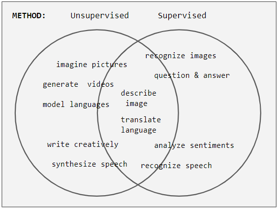
Comparison to supervised learning

The fundamental difference: unsupervised learning works with unlabeled data, while supervised learning requires labeled training examples (input-output pairs).

• Supervised learning aims to predict specific outputs (e.g., "this image contains a pedestrian"). Unsupervised learning discovers inherent structures (e.g., "these images share similar visual features").
• Unsupervised methods often serve as preprocessing steps for supervised tasks. For example, you might use PCA to reduce feature dimensionality before training a classifier.
• Evaluating unsupervised models is harder because there are no ground truth labels to compare against. You have to rely on internal metrics like silhouette scores or domain expert judgment.

Applications in computer vision

• Image segmentation groups pixels into meaningful regions or objects without needing per-pixel labels
• Feature learning extracts relevant visual representations from raw image data, which can then feed into downstream tasks
• Anomaly detection identifies unusual patterns or objects in images, useful in manufacturing inspection or medical imaging
• Generative modeling creates new, realistic images by learning the underlying data distribution

Clustering algorithms

Clustering algorithms group similar data points together based on their features. In computer vision, this translates to segmenting images into regions, grouping visually similar objects, and organizing large image datasets. The choice of algorithm depends on the shape of your clusters, the noise level in your data, and whether you know how many clusters to expect.

K-means clustering

K-means partitions data into $K$ predefined clusters by minimizing within-cluster variance. It's one of the simplest and most widely used clustering algorithms.

The algorithm works as follows:

1. Initialize $K$ cluster centroids randomly
2. Assign each data point to the nearest centroid (using Euclidean distance)
3. Recalculate each centroid as the mean of all points assigned to it
4. Repeat steps 2-3 until assignments stop changing (convergence)

K-means is commonly used for color quantization, where you reduce the number of colors in an image. For example, you could represent a photo using only 16 colors by running K-means with $K = 16$ on the pixel color values.

Watch out for two weaknesses: K-means is sensitive to initial centroid placement (which is why K-means++ initialization is often preferred), and it struggles with outliers that can pull centroids away from the true cluster centers.

Hierarchical clustering

Hierarchical clustering builds a tree-like structure of nested clusters called a dendrogram. You can cut the dendrogram at different levels to get different numbers of clusters, which gives you a multi-scale view of the data.

There are two main approaches:

• Agglomerative (bottom-up): Start with each data point as its own cluster, then repeatedly merge the two closest clusters until everything is in one cluster.
• Divisive (top-down): Start with all points in one cluster and recursively split.

Agglomerative clustering steps:

1. Treat each data point as a separate cluster
2. Compute distances between all pairs of clusters
3. Merge the two closest clusters
4. Repeat steps 2-3 until all points belong to a single cluster

This approach is useful for hierarchical image segmentation, where you might want to see an image decomposed at multiple levels of detail, from fine-grained regions to large object parts.

DBSCAN algorithm

DBSCAN (Density-Based Spatial Clustering of Applications with Noise) groups together points that are densely packed and marks points in sparse regions as outliers.

It requires two parameters:

• Epsilon ($\epsilon$): the radius of the neighborhood around each point
• minPoints: the minimum number of points required within that radius to form a dense region

Key advantages over K-means:

• Discovers clusters of arbitrary shape (not just spherical)
• Robust to noise and outliers, which it explicitly labels
• Does not require you to specify the number of clusters in advance

DBSCAN is particularly useful for object detection in complex scenes where objects have irregular shapes and the background contains noise.

Dimensionality reduction techniques

Images are inherently high-dimensional. A modest 256×256 grayscale image has 65,536 dimensions (one per pixel). Dimensionality reduction transforms this high-dimensional data into lower-dimensional representations while preserving the most important visual information. This makes processing, visualization, and analysis far more tractable.

Principal Component Analysis (PCA)

PCA is a linear technique that finds the directions of maximum variance in the data and projects onto those directions. These directions are called principal components.

Steps to perform PCA:

1. Standardize the data (zero mean, unit variance per feature)
2. Compute the covariance matrix of the standardized data
3. Calculate the eigenvectors and eigenvalues of the covariance matrix
4. Sort eigenvectors by decreasing eigenvalue (the eigenvalue tells you how much variance that component captures)
5. Project the data onto the top $k$ eigenvectors to get a $k$-dimensional representation

PCA is used for feature extraction, image compression, and face recognition (where it's historically known as "Eigenfaces"). Its main limitation is that it can only capture linear relationships in the data.

t-SNE

t-Distributed Stochastic Neighbor Embedding (t-SNE) is a non-linear technique designed primarily for visualizing high-dimensional data in 2D or 3D.

The algorithm:

1. Computes pairwise similarities between points in the original high-dimensional space (using Gaussian distributions)
2. Initializes a random low-dimensional embedding
3. Iteratively adjusts the embedding to minimize the Kullback-Leibler divergence between the high-dimensional similarity distribution and the low-dimensional one (which uses a Student's t-distribution)

t-SNE excels at preserving local structure, meaning nearby points in high-dimensional space stay nearby in the visualization. This makes it great for revealing clusters in image datasets and understanding what a model's feature space looks like.

The tradeoff: t-SNE is computationally expensive for large datasets and doesn't preserve global distances well. It's a visualization tool, not a general-purpose dimensionality reduction method for downstream tasks.

Autoencoders for dimensionality reduction

An autoencoder is a neural network trained to compress input data into a lower-dimensional latent space and then reconstruct the original input from that compressed representation.

The architecture has two parts:

• Encoder: maps the input to a lower-dimensional latent representation
• Decoder: reconstructs the input from the latent representation

Training minimizes the reconstruction error (typically mean squared error between input and output). The bottleneck in the middle forces the network to learn a compact representation that captures the most important features.

Variants include:

• Denoising autoencoders: trained to reconstruct clean inputs from corrupted versions, which encourages more robust features
• Variational autoencoders (VAEs): add a probabilistic structure to the latent space (covered in more detail under generative models)

Applications include image compression, feature learning, and anomaly detection.

Feature extraction methods

Feature extraction identifies distinctive characteristics or patterns in image data that can be used for recognition, matching, and retrieval. Good features should be discriminative (different for different objects) and robust to changes in scale, rotation, and lighting.

SIFT and SURF

SIFT (Scale-Invariant Feature Transform) and SURF (Speeded Up Robust Features) are local feature descriptors designed to be robust to scale, rotation, and illumination changes.

SIFT works in four stages:

1. Scale-space extrema detection: Find candidate keypoints by looking for local extrema across different scales using Difference-of-Gaussians
2. Keypoint localization: Refine keypoint positions and discard low-contrast or edge-like points
3. Orientation assignment: Assign a dominant orientation to each keypoint based on local gradient directions
4. Descriptor generation: Build a 128-dimensional descriptor from gradient histograms around the keypoint

SURF achieves similar results faster by using integral images and box filters instead of Gaussians. Both are widely applied in image matching, object recognition, and 3D reconstruction.

HOG descriptors

Histogram of Oriented Gradients (HOG) captures local shape information by computing gradient orientations in image patches. The idea is that the distribution of gradient directions describes the shape of edges and contours.

HOG computation:

1. Divide the image into small spatial regions called cells
2. Compute gradient magnitude and orientation for each pixel in each cell
3. Build a histogram of gradient orientations for each cell (typically 9 orientation bins)
4. Normalize histograms across larger blocks of cells to account for illumination variation

HOG became famous for pedestrian detection and remains useful for object recognition. It's robust to small geometric transformations and lighting changes because the normalization step handles local contrast variation.

Convolutional features

Features extracted from convolutional neural networks (CNNs) trained on large datasets like ImageNet have become the dominant approach in modern computer vision.

CNNs learn a hierarchical representation of visual information:

• Lower layers capture low-level features like edges and textures
• Middle layers capture parts and patterns
• Higher layers represent more abstract concepts like objects and scenes

Transfer learning takes features from a CNN pre-trained on one task and applies them to a different task. This works because the lower and middle layers learn general visual features that transfer well across domains. Feature visualization techniques (like activation maximization) can reveal what patterns each layer has learned.

Generative models

Generative models learn the underlying probability distribution of training data so they can generate new samples that look like they came from the same distribution. In computer vision, this means creating realistic images, translating between image domains, and learning useful visual representations.

Gaussian Mixture Models (GMMs)

A GMM represents data as a weighted combination of multiple Gaussian distributions. Each Gaussian component has its own mean, covariance, and mixing coefficient (the weight indicating how much that component contributes).

Training uses the Expectation-Maximization (EM) algorithm:

1. Initialize the parameters (means, covariances, mixing coefficients)
2. E-step: For each data point, compute the probability that it belongs to each Gaussian component (these are called responsibilities)
3. M-step: Update each component's parameters using the responsibilities as weights
4. Repeat steps 2-3 until the parameters converge

GMMs are applied in image segmentation (modeling pixel color distributions), background modeling (separating foreground from background in video), and color clustering. They're more flexible than K-means because each cluster can have its own shape and size via the covariance matrix.

Variational Autoencoders (VAEs)

A VAE combines the autoencoder architecture with probabilistic (variational) inference. Unlike a standard autoencoder, the encoder outputs parameters of a probability distribution (typically a Gaussian mean and variance) rather than a single point in latent space.

The training objective balances two terms:

1. Reconstruction loss: How well the decoder reconstructs the input from a sample drawn from the latent distribution
2. KL divergence: Regularizes the latent space by encouraging it to stay close to a prior distribution (usually a standard Gaussian $\mathcal{N}(0, I)$)

Because the latent space is continuous and regularized, you can generate new images by sampling from the prior and passing samples through the decoder. You can also interpolate smoothly between images by interpolating in latent space. VAEs are used for image generation, data augmentation, and representation learning.

Generative Adversarial Networks (GANs)

A GAN trains two neural networks against each other in an adversarial process:

1. Generator: Takes random noise as input and produces fake images, trying to fool the discriminator
2. Discriminator: Receives both real images and the generator's fakes, trying to correctly classify which is which

During training, the generator minimizes the probability that the discriminator correctly identifies its outputs as fake, while the discriminator maximizes its classification accuracy. This adversarial dynamic pushes the generator to produce increasingly realistic images.

Notable variants include:

• DCGAN: Uses deep convolutional architectures for both generator and discriminator
• StyleGAN: Introduces style-based generation for high-quality, controllable image synthesis
• CycleGAN: Enables unpaired image-to-image translation (e.g., converting photos to paintings without paired examples)

GANs are applied in high-resolution image synthesis, image-to-image translation, super-resolution, and data augmentation.

Anomaly detection

Anomaly detection identifies samples that deviate significantly from normal patterns. In computer vision, this means flagging defective products on an assembly line, detecting suspicious activity in surveillance footage, or identifying abnormal regions in medical scans. A key property of these methods is that they typically train only on normal data, then flag anything that doesn't fit.

One-class SVM

One-class SVM is a Support Vector Machine variant designed for anomaly detection. Instead of separating two classes, it learns a boundary that encloses the majority of normal data points.

The training process:

1. Map data points to a high-dimensional feature space (using a kernel function)
2. Find the smallest hypersphere (or hyperplane with maximum margin from the origin) that contains most of the data
3. Use the kernel trick to handle non-linear decision boundaries without explicitly computing the high-dimensional mapping

New samples falling outside the learned boundary are classified as anomalies. One-class SVM is effective for novelty detection in image data and identifying defects in visual inspection tasks.

Isolation Forest

Isolation Forest is an ensemble method built on a simple insight: anomalies are rare and different, so they're easier to isolate through random partitioning.

The algorithm:

1. Randomly select a feature and a split value within that feature's range
2. Recursively partition the data using random splits until each point is isolated in its own partition
3. Compute an anomaly score based on the average path length needed to isolate each point

Points that require fewer splits to isolate (shorter path lengths) are more likely to be anomalies. This is because outliers sit in sparse regions and get separated quickly.

Advantages:

• Handles high-dimensional data efficiently
• Robust to irrelevant features
• Scales well to large datasets

It's applied in detecting unusual objects or regions in images and video frames.

Autoencoders for anomaly detection

This approach uses the reconstruction error of an autoencoder as an anomaly signal. The logic: if you train an autoencoder only on normal data, it'll learn to reconstruct normal patterns well but struggle with anomalous inputs.

The process:

1. Train an autoencoder exclusively on normal data samples
2. For each new sample, compute the reconstruction error (difference between input and reconstructed output)
3. Samples with reconstruction error above a threshold are classified as anomalies

This works because the autoencoder's latent space captures the structure of normal data. Anomalous inputs don't fit that structure, so they reconstruct poorly. Variants like denoising autoencoders and variational autoencoders can improve robustness. This approach is particularly effective in medical imaging and industrial inspection, where anomalies are rare and diverse.

Self-organizing maps

Self-organizing maps (SOMs) create low-dimensional (typically 2D) representations of high-dimensional data while preserving topological relationships. Points that are similar in the original space end up near each other on the map. This makes SOMs useful for both visualization and clustering of complex image features.

Kohonen networks

A Kohonen network is the neural network architecture that implements a SOM. It consists of a grid of neurons, where each neuron has an associated weight vector with the same dimensionality as the input data.

Training process:

1. Initialize neuron weights randomly
2. Present an input vector to the network
3. Find the Best Matching Unit (BMU): the neuron whose weight vector is most similar to the input
4. Update the BMU and its neighbors' weights to move closer to the input (the neighborhood size and learning rate decrease over time)
5. Repeat steps 2-4 for all inputs across multiple epochs

After training, the resulting map is a non-linear projection of the input space. Neurons that are close together on the grid respond to similar input patterns, creating a topology-preserving map.

Applications in image processing

• Color quantization: Reduces the number of colors in an image while preserving visual quality by mapping pixel colors onto SOM neurons
• Texture analysis: Groups similar textures and identifies dominant patterns across an image dataset
• Image compression: Represents images using a reduced set of SOM neuron weight vectors as a codebook
• Feature extraction: Creates low-dimensional representations of image patches or regions for downstream tasks
• Image segmentation: Clusters pixels or regions based on their similarity as mapped onto the SOM grid

Evaluation metrics

Evaluating unsupervised learning is inherently tricky because there are no ground truth labels to compare against. Instead, you rely on internal metrics that measure properties like cluster compactness and separation. These metrics help you compare different algorithms or tune hyperparameters (like the number of clusters).

Silhouette score

The silhouette score measures how similar each data point is to its own cluster compared to the nearest neighboring cluster.

For a single sample, the silhouette coefficient is:

$s = \frac{b - a}{\max(a, b)}$

where $a$ is the mean distance from the point to other points in the same cluster (intra-cluster distance) and $b$ is the mean distance to points in the nearest different cluster.

• Range: -1 to 1
• Values near +1 mean the point is well-matched to its own cluster and poorly matched to neighboring clusters
• Values near 0 mean the point sits on the boundary between clusters
• Negative values mean the point may be assigned to the wrong cluster

The overall silhouette score (averaged across all points) is used to evaluate image segmentation and object clustering results.

Davies-Bouldin index

The Davies-Bouldin index measures the ratio of within-cluster scatter to between-cluster separation. Lower values indicate better clustering.

$DB = \frac{1}{n} \sum_{i=1}^n \max_{j \neq i} \left( \frac{\sigma_i + \sigma_j}{d(c_i, c_j)} \right)$

where $n$ is the number of clusters, $\sigma_i$ is the average distance of points in cluster $i$ to its centroid, and $d(c_i, c_j)$ is the distance between the centroids of clusters $i$ and $j$.

The formula finds the worst-case pair for each cluster (the neighboring cluster it's most similar to) and averages across all clusters. It evaluates both compactness within clusters and separation between them.

Calinski-Harabasz index

The Calinski-Harabasz index (also called the Variance Ratio Criterion) measures the ratio of between-cluster dispersion to within-cluster dispersion. Higher values indicate better-defined clusters.

$CH = \frac{tr(B_k)}{tr(W_k)} \times \frac{n - k}{k - 1}$

where $tr(B_k)$ is the trace of the between-cluster scatter matrix, $tr(W_k)$ is the trace of the within-cluster scatter matrix, $n$ is the total number of data points, and $k$ is the number of clusters.

The $\frac{n - k}{k - 1}$ term adjusts for the number of clusters (adding more clusters trivially reduces within-cluster scatter). This metric works well for convex, roughly spherical clusters and is computationally efficient, making it practical for evaluating clustering results on large image datasets.

Challenges and limitations

Understanding the limitations of unsupervised learning helps you choose the right method and set realistic expectations for what these algorithms can achieve.

Curse of dimensionality

The curse of dimensionality refers to problems that emerge as the number of features grows. In high-dimensional spaces:

• Data points become increasingly sparse, making it hard to find meaningful clusters
• Distance metrics lose their discriminative power (all points become roughly equidistant)
• Computational complexity grows, sometimes exponentially

This is a real problem in image analysis because raw pixel data is extremely high-dimensional. A 1024×1024 RGB image has over 3 million dimensions. Dimensionality reduction techniques like PCA and t-SNE, along with learned feature extractors like autoencoders and CNNs, are the primary tools for mitigating this issue.

Interpretation of results

Unsupervised learning produces results that often require expert interpretation. Without labels, there's no automatic way to know what a discovered cluster "means."

Specific challenges in computer vision:

• Assigning semantic meaning to discovered clusters or features (does cluster 3 represent "outdoor scenes" or is it just grouping by dominant color?)
• Validating the relevance of extracted patterns without ground truth
• Explaining the internal workings of complex models like GANs

Visualization techniques and domain expertise are essential for making sense of unsupervised learning outputs.

Scalability issues

Many unsupervised algorithms struggle with large-scale image datasets:

• Computational complexity: Algorithms like hierarchical clustering have $O(n^2)$ or worse time complexity
• Memory limitations: Storing pairwise distance matrices for large datasets can exceed available RAM
• High-resolution data: Processing high-resolution images or video streams demands significant resources

Approaches to address scalability include distributed computing, mini-batch variants of algorithms (like mini-batch K-means), online/incremental learning, and approximate nearest neighbor methods. There's almost always a tradeoff between accuracy and computational efficiency.

Recent advancements

Recent work has pushed unsupervised and self-supervised methods to the point where they can rival supervised approaches on many benchmarks, dramatically reducing the need for labeled data.

Self-supervised learning

Self-supervised learning creates supervised training signals from the data itself by designing pretext tasks that require understanding visual structure.

Common pretext tasks in computer vision:

• Rotation prediction: Rotate an image by 0°, 90°, 180°, or 270° and train the network to predict which rotation was applied
• Jigsaw puzzle solving: Shuffle image patches and train the network to predict the correct arrangement
• Colorization: Convert images to grayscale and train the network to predict the original colors

The network learns rich visual representations while solving these tasks, and those representations transfer well to downstream tasks like classification and detection, even with limited labeled data.

Contrastive learning

Contrastive learning trains a model to pull similar (positive) pairs close together in feature space while pushing dissimilar (negative) pairs apart.

Popular methods:

• SimCLR: Creates positive pairs by applying different random augmentations (crop, color jitter, blur) to the same image. All other images in the batch serve as negatives.
• MoCo (Momentum Contrast): Maintains a large, dynamically updated dictionary of negative samples using a momentum-updated encoder, allowing larger effective batch sizes.
• BYOL (Bootstrap Your Own Latent): Learns from positive pairs only, without needing explicit negative samples, using a momentum-updated target network.

These methods have achieved results competitive with supervised pre-training on tasks like image retrieval, object detection, and semantic segmentation.

Few-shot learning approaches

Few-shot learning aims to recognize new categories from just a handful of labeled examples. Unsupervised techniques contribute in several ways:

• Meta-learning algorithms learn a learning procedure that generalizes to new tasks with minimal data
• Prototypical networks represent each class by a prototype (mean embedding) in feature space and classify by nearest prototype, leveraging unsupervised clustering principles
• Generative data augmentation uses GANs or VAEs to synthesize additional training examples for rare classes

These approaches are valuable when you need to recognize objects from categories with very few available examples, combining the strengths of both supervised and unsupervised learning.