3.3 Blob detection

Definition of blob detection

Blob detection identifies regions in a digital image whose properties differ noticeably from their surroundings. A "blob" is essentially a patch of pixels that share similar brightness or color, standing out against the neighboring area. This makes blob detection one of the core tools in computer vision: it lets you isolate distinct objects or features before doing any higher-level analysis like recognition or tracking.

Importance in image processing

Blob detection matters because it bridges the gap between raw pixel data and meaningful image understanding. By isolating candidate regions, it enables:

• Object recognition by separating potential objects of interest from the background
• Feature extraction for downstream tasks like object tracking and image segmentation
• Automated analysis in domains like medical imaging (finding tumors or cell nuclei), industrial quality control (spotting defects), and satellite imagery interpretation

Blob detection algorithms

Several mathematical approaches exist for finding blobs, and they differ in how sensitive they are to blob shape, size, and intensity profile. Choosing the right one depends on your application and what kind of blobs you expect to find.

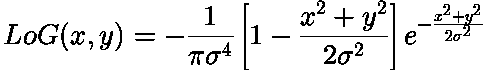
Laplacian of Gaussian (LoG)

The LoG method works in two stages. First, it smooths the image with a Gaussian filter to suppress noise. Then it applies the Laplacian operator, which highlights regions of rapid intensity change. Blob centers show up as local maxima or minima in the LoG response.

The LoG kernel for a 2D image is:

$\nabla^2 G(x,y) = \frac{x^2 + y^2 - 2\sigma^2}{\sigma^4} \, e^{-\frac{x^2 + y^2}{2\sigma^2}}$

where $\sigma$ controls the scale of the Gaussian smoothing. Larger $\sigma$ values detect larger blobs.

LoG is particularly effective for circular or elliptical blobs with smooth intensity profiles, but it's computationally expensive since you need to convolve the image with the full LoG kernel at each scale.

Difference of Gaussians (DoG)

DoG approximates the LoG by simply subtracting two Gaussian-blurred versions of the same image, each blurred with a different $\sigma$:

$DoG(x,y,\sigma) = G(x,y, k\sigma) - G(x,y, \sigma)$

Here $G$ is the Gaussian function and $k$ is a constant scaling factor (typically around 1.6). Blobs appear at local extrema in the resulting difference image.

The key advantage of DoG over LoG is computational efficiency. Since you're reusing Gaussian-blurred images that you'd likely compute anyway (for example, in a scale-space pyramid), DoG avoids the cost of computing second derivatives directly. This is why SIFT uses DoG internally for its keypoint detection.

Determinant of Hessian (DoH)

The Hessian-based approach uses the matrix of second-order partial derivatives at each pixel:

$H = \begin{bmatrix} \frac{\partial^2 f}{\partial x^2} & \frac{\partial^2 f}{\partial x \partial y} \\ \frac{\partial^2 f}{\partial y \partial x} & \frac{\partial^2 f}{\partial y^2} \end{bmatrix}$

The blob response at each pixel is the determinant of this matrix:

$R = \det(H) = \frac{\partial^2 f}{\partial x^2} \frac{\partial^2 f}{\partial y^2} - \left(\frac{\partial^2 f}{\partial x \partial y}\right)^2$

A large positive determinant indicates a blob-like structure (the intensity curves in both directions). Unlike LoG, the Hessian approach can detect blobs of various shapes and orientations, not just circular ones. SURF uses an approximated version of this method with box filters for speed.

Scale-space representation

Real images contain blobs of many different sizes, so you can't just pick a single $\sigma$ and call it done. Scale-space representation solves this by creating a stack of progressively blurred images:

$L(x,y,\sigma) = G(x,y,\sigma) * I(x,y)$

where $I$ is the input image and $*$ denotes convolution. Each layer in the stack corresponds to a different $\sigma$ value. You then search for blob responses that are extrema not just in the spatial $(x,y)$ dimensions but also across scales. This is what makes blob detection scale-invariant, meaning it can find the same object whether it appears large (close to the camera) or small (far away).

Blob detection steps

Image preprocessing

Before running any blob detector, you typically need to clean up the input:

1. Noise reduction: Apply Gaussian smoothing or median filtering to reduce spurious detections
2. Contrast enhancement: Use histogram equalization or normalization to make blobs stand out from the background
3. Color conversion: Convert to grayscale if you're using an intensity-based detector, or choose an appropriate color space (HSV, Lab) if color matters

Blob candidate identification

This is where the actual detection happens:

1. Apply your chosen algorithm (LoG, DoG, or DoH) to the preprocessed image, producing a blob response map
2. Find local extrema in the response map; these are your candidate blob locations
3. Apply a threshold to discard weak responses that are likely noise
4. Run non-maximum suppression to eliminate overlapping detections and pinpoint blob centers

Blob verification

Not every candidate is a real blob. Verification refines the results:

1. Filter candidates by size, shape, or intensity profile to match expected blob characteristics
2. Apply morphological operations (erosion, dilation) to clean up blob boundaries
3. Merge overlapping blobs or split large regions that contain multiple blobs
4. Validate remaining detections against predefined constraints or a learned model

Feature descriptors for blobs

Once you've detected blobs, you need a way to describe them quantitatively so you can match, classify, or track them. Common descriptor types include:

• Shape descriptors: area, perimeter, circularity ($4\pi \cdot \text{area} / \text{perimeter}^2$), aspect ratio
• Intensity-based descriptors: mean, variance, and histogram of pixel values within the blob
• Texture descriptors: Gray-Level Co-occurrence Matrix (GLCM) or Local Binary Patterns (LBP) capture local texture patterns inside the blob
• Moment-based descriptors: Hu moments and Zernike moments provide representations that are invariant to rotation and scale, making them useful for matching blobs across different views

Applications of blob detection

Object detection

Blob detection is a natural fit for finding compact, well-defined objects in cluttered scenes. Traffic signs, cells in microscopy images, and fruit on a conveyor belt are all examples where blob-based approaches work well. Typically you combine blob detection with a classifier to not just find blobs but identify what they are. In video, blob detection enables real-time object detection for surveillance and autonomous systems.

Tracking

In video analysis, blob detection identifies moving objects frame by frame. The centroid of each detected blob serves as a feature point that tracking algorithms like Kalman filters or particle filters can follow over time. This supports multi-object tracking in crowded scenes and has applications in sports analysis, traffic monitoring, and human behavior understanding.

Medical imaging

Blob detection is heavily used in medical imaging to find anatomical structures and abnormalities. It can detect lesions and tumors in MRI or CT scans, identify cell nuclei in microscopy images, and highlight regions of interest for radiologists. This forms the backbone of many computer-aided diagnosis systems and enables quantitative measurements that support clinical decision-making.

Challenges in blob detection

Noise sensitivity

Image noise creates false intensity variations that blob detectors can mistake for real blobs, or that can mask true blobs. Careful preprocessing helps, but there's always a tradeoff: too much smoothing removes noise but also blurs small blobs. Adaptive thresholding and algorithms that explicitly model noise characteristics can improve robustness.

Scale selection

Choosing the right scale parameters is tricky. If your $\sigma$ range is too narrow, you'll miss blobs outside that size range. Multi-scale approaches cover more ground but increase computation and can introduce ambiguities when the same blob produces responses at multiple scales. Automatic scale selection (finding extrema across scale space) addresses this, but adds complexity.

Computational complexity

LoG and Hessian-based methods involve computing second-order derivatives at multiple scales, which gets expensive for high-resolution images or real-time video. Common optimizations include:

• Integral images for fast box filter computation
• Image pyramids to process downsampled versions at coarser scales
• GPU acceleration for parallel processing
• Approximation methods like those used in SURF, which trade a small amount of accuracy for significant speed gains

Blob detection vs. edge detection

These two techniques are complementary, not competing. Edge detection (Canny, Sobel) finds boundaries by looking for sharp intensity gradients at individual pixels. Blob detection finds regions by looking for areas of consistent intensity that differ from their surroundings.

• Edge detection is better for shape analysis and contour extraction
• Blob detection is better for finding compact objects and regions of interest
• Many practical systems combine both: use blob detection to find candidate regions, then use edge detection to refine their boundaries

Performance evaluation metrics

To measure how well a blob detector performs, you need ground-truth annotations to compare against:

• Precision: fraction of detected blobs that are actually real blobs (how many detections are correct)
• Recall: fraction of real blobs that were successfully detected (how many true blobs you found)
• F1-score: harmonic mean of precision and recall, giving a single balanced metric
• Intersection over Union (IoU): measures spatial overlap between detected and ground-truth blob regions; an IoU above 0.5 is a common threshold for counting a detection as correct
• ROC curves: plot true positive rate vs. false positive rate across different detection thresholds, showing overall detector performance

Optimization techniques

• Integral images let you compute box filter responses in constant time regardless of filter size, enabling fast approximations of Gaussian kernels
• Fast Hessian detector (used in SURF) replaces Gaussian second derivatives with box filter approximations
• Pyramid representations reduce computation by running detection on progressively downsampled images for coarser scales
• Parallel processing on multi-core CPUs or GPUs speeds up the per-pixel computations that dominate blob detection
• Approximate methods like those in SURF and FAST trade some detection accuracy for major speed improvements, making real-time applications feasible

Blob detection in color images

Standard blob detection operates on single-channel (grayscale) images, but extending it to color images can capture richer information. The choice of color space matters: RGB is straightforward but sensitive to lighting changes, while HSV and Lab separate intensity from color, which can improve robustness.

Color blob detection is useful when blobs are defined by their color rather than just intensity, such as detecting traffic lights, colored markers, or specific biological stains in microscopy. The main challenge is maintaining color consistency under varying illumination conditions.

Machine learning approaches

Convolutional neural networks

CNNs can learn to detect blobs directly from training data, bypassing hand-crafted feature design. Architectures like U-Net (originally designed for biomedical image segmentation) are well-suited for blob detection tasks because they produce pixel-level predictions. Transfer learning lets you adapt a pre-trained network to your specific blob detection problem even with limited training data. Attention mechanisms can further improve performance by focusing the network on relevant image regions.

Deep learning models

Beyond standard CNNs, several other deep learning paradigms apply to blob detection:

• GANs can generate synthetic blob images for data augmentation when labeled training data is scarce
• Autoencoders enable unsupervised blob detection by learning to reconstruct normal images and flagging regions with high reconstruction error as anomalies
• Reinforcement learning can adaptively tune detection parameters based on feedback
• Graph neural networks model spatial relationships between detected blobs, useful when blob arrangements carry meaning
• Few-shot learning addresses scenarios where you have very few labeled examples of the blob type you're looking for

Blob detection libraries

OpenCV implementations

OpenCV provides several ready-to-use blob detection tools:

• cv2.SimpleBlobDetector is the most common starting point. You configure it through cv2.SimpleBlobDetector_Params, which lets you set thresholds for area, circularity, convexity, and inertia ratio.
• MSER (Maximally Stable Extremal Regions) detects blob-like regions based on intensity thresholding stability and is available via cv2.MSER_create().
• GPU-accelerated versions are available in OpenCV's CUDA module for performance-critical applications.

MATLAB functions

• detectBLOBFeatures implements multiscale blob detection using the SURF-inspired approach
• vision.BlobAnalysis is a System object for real-time blob analysis and measurement
• bwconncomp and regionprops handle connected component labeling and blob property extraction on binary images
• The Image Processing Toolbox and Parallel Computing Toolbox provide additional functions for blob refinement and distributed processing on large datasets

Future trends in blob detection

• Deep learning integration: Combining classical blob detectors with learned features for better accuracy and adaptability
• Real-time high-resolution processing: Developing algorithms fast enough for 4K video and beyond
• 3D blob detection: Extending techniques to volumetric data for medical imaging (CT/MRI volumes) and 3D computer vision
• Context-aware detection: Using scene understanding to improve blob detection by considering spatial relationships between objects
• Multi-modal fusion: Combining data from different sensor types (RGB-D cameras, hyperspectral sensors) to detect blobs that are invisible in any single modality