7.1 Probability and random variables

Probability and random variables form the backbone of statistical signal processing. They provide the mathematical framework for analyzing signals with unpredictable components, letting you model noise, interference, and other stochastic phenomena that show up in real-world data.

This section covers probability theory foundations, types of random variables and their distributions, expectation and moments, and multivariate random variables.

Probability theory foundations

Probability theory gives you the formal tools to reason about uncertainty. In signal processing, signals are almost always corrupted by noise or other random effects, so you need a rigorous way to describe and manipulate randomness before you can build estimators, detectors, or filters.

Experiments, sample spaces and events

• An experiment is any procedure whose outcome is determined by chance (transmitting a bit over a noisy channel, measuring a voltage).
• The sample space $\Omega$ is the set of all possible outcomes of that experiment.
• An event is a subset of $\Omega$. For example, if you roll a die, the event "even number" is the subset $\{2, 4, 6\}$.

Axioms of probability

All of probability is built on three axioms (Kolmogorov's axioms):

1. Non-negativity: $P(A) \geq 0$ for any event $A$.
2. Normalization: $P(\Omega) = 1$.
3. Countable additivity: For mutually exclusive events $A_1, A_2, \ldots$,

$P\left(\bigcup_{i=1}^{\infty} A_i\right) = \sum_{i=1}^{\infty} P(A_i)$

Every probability rule you'll use downstream (complement rule, inclusion-exclusion, etc.) derives from these three.

Conditional probability

Conditional probability captures how the probability of event $A$ changes once you know event $B$ has occurred:

$P(A|B) = \frac{P(A \cap B)}{P(B)}, \quad P(B) > 0$

This is central to signal processing. For instance, you might want the probability that a transmitted symbol was "1" given a particular received voltage. Conditioning on observed data is the starting point for all Bayesian estimation.

Statistical independence

Two events $A$ and $B$ are statistically independent if knowing one tells you nothing about the other. The formal condition is:

$P(A \cap B) = P(A)P(B)$

Equivalently, $P(A|B) = P(A)$. Independence is a powerful simplifying assumption. In many signal processing models, noise samples are assumed independent of the signal and of each other, which makes joint probabilities factor into products.

Bayes' theorem applications

Bayes' theorem lets you invert a conditional probability:

$P(A|B) = \frac{P(B|A)\,P(A)}{P(B)}$

• $P(A)$ is the prior (what you believed before observing data).
• $P(B|A)$ is the likelihood (how probable the observed data is under hypothesis $A$).
• $P(A|B)$ is the posterior (your updated belief after seeing data).

In signal processing, Bayes' theorem underpins MAP and MMSE estimation, hypothesis testing, and signal detection in noise.

Random variables

A random variable is a function that maps each outcome in $\Omega$ to a real number. It bridges the abstract sample space and the numerical quantities you actually compute with. Virtually every signal processing model represents signals, noise, and parameters as random variables.

Discrete vs continuous types

• Discrete random variables take on a countable set of values (e.g., the number of bit errors in a packet).
• Continuous random variables can take any value in an interval (e.g., the amplitude of thermal noise).

The distinction matters because discrete variables use sums and PMFs, while continuous variables use integrals and PDFs.

Probability mass functions (PMFs)

For a discrete random variable $X$, the PMF $p_X(x)$ gives the probability that $X$ equals $x$:

$p_X(x) = P(X = x)$

Two requirements: $p_X(x) \geq 0$ for all $x$, and $\sum_x p_X(x) = 1$. You use the PMF to compute expectations, probabilities of events, and other statistics for discrete quantities.

Cumulative distribution functions (CDFs)

The CDF works for both discrete and continuous random variables:

$F_X(x) = P(X \leq x)$

• Discrete case: $F_X(x) = \sum_{t \leq x} p_X(t)$
• Continuous case: $F_X(x) = \int_{-\infty}^{x} f_X(t)\, dt$

The CDF is always non-decreasing, right-continuous, and satisfies $F_X(-\infty) = 0$ and $F_X(\infty) = 1$. It's especially useful for computing probabilities like $P(a < X \leq b) = F_X(b) - F_X(a)$.

Probability density functions (PDFs)

For a continuous random variable $X$, the PDF $f_X(x)$ is the derivative of the CDF:

$f_X(x) = \frac{dF_X(x)}{dx}$

The PDF itself is not a probability (it can exceed 1), but integrating it over an interval gives a probability:

$P(a \leq X \leq b) = \int_a^b f_X(x)\, dx$

Requirements: $f_X(x) \geq 0$ and $\int_{-\infty}^{\infty} f_X(x)\, dx = 1$.

Joint probability distributions

When you have two or more random variables, their joint distribution describes their simultaneous behavior.

• Discrete: joint PMF $p_{X,Y}(x,y) = P(X=x, Y=y)$
• Continuous: joint PDF $f_{X,Y}(x,y)$, where $P((X,Y) \in A) = \iint_A f_{X,Y}(x,y)\, dx\, dy$

Joint distributions are essential for studying how signal components relate to each other, such as the in-phase and quadrature components of a complex baseband signal.

Expectation and moments

Moments summarize the shape of a distribution with a few numbers. The mean tells you where the distribution is centered, the variance tells you how spread out it is, and higher moments capture asymmetry and tail behavior.

Expected value of a random variable

The expected value (mean) of $X$ is:

• Discrete: $E[X] = \sum_x x\, p_X(x)$
• Continuous: $E[X] = \int_{-\infty}^{\infty} x\, f_X(x)\, dx$

The expected value is linear: $E[aX + bY] = aE[X] + bE[Y]$, regardless of whether $X$ and $Y$ are independent. This linearity property is used constantly in signal processing derivations.

Variance and standard deviation

Variance measures dispersion around the mean:

$\text{Var}(X) = E[(X - E[X])^2] = E[X^2] - (E[X])^2$

The second form is often easier to compute. The standard deviation $\sigma_X = \sqrt{\text{Var}(X)}$ has the same units as $X$, making it more interpretable. In signal processing, variance of noise directly determines signal-to-noise ratio.

Moments and moment-generating functions

The $n$-th moment of $X$ is $E[X^n]$. The $n$-th central moment is $E[(X - E[X])^n]$. The first moment is the mean; the second central moment is the variance.

The moment-generating function (MGF) compactly encodes all moments:

$M_X(t) = E[e^{tX}]$

You recover moments by differentiation: $E[X^n] = M_X^{(n)}(0)$. The MGF uniquely determines the distribution (when it exists in a neighborhood of $t=0$), and it's particularly convenient for finding the distribution of sums of independent random variables since $M_{X+Y}(t) = M_X(t) M_Y(t)$.

Characteristic functions

The characteristic function (CF) is the Fourier-domain counterpart of the MGF:

$\phi_X(t) = E[e^{itX}]$

Unlike the MGF, the CF always exists. It uniquely determines the distribution and shares the multiplication property for sums of independent variables. If you're comfortable with Fourier transforms from earlier signal processing courses, the CF will feel natural: it is the Fourier transform of the PDF.

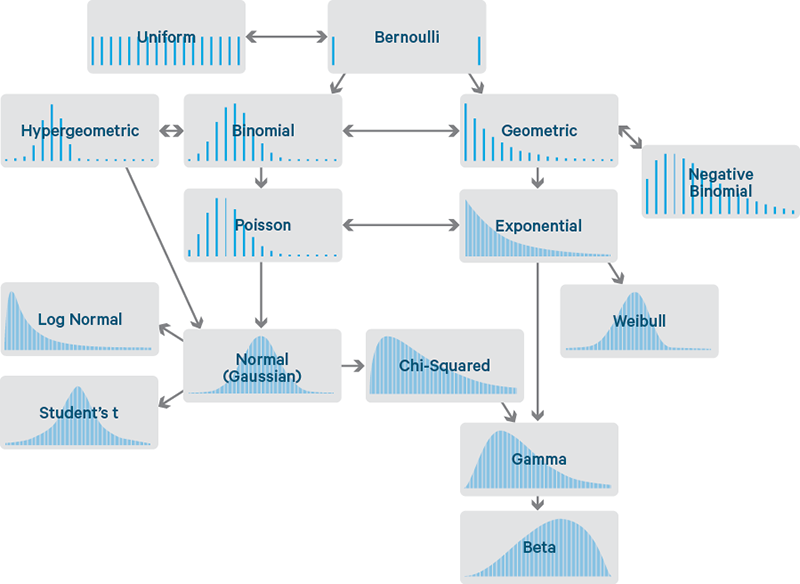
Common discrete distributions

Bernoulli and binomial distributions

A Bernoulli random variable models a single trial: success ($X=1$) with probability $p$, failure ($X=0$) with probability $1-p$. Mean: $p$. Variance: $p(1-p)$.

The binomial distribution counts the number of successes in $n$ independent Bernoulli trials:

$p_X(k) = \binom{n}{k} p^k (1-p)^{n-k}, \quad k = 0, 1, \ldots, n$

Mean: $np$. Variance: $np(1-p)$. A typical application is counting bit errors in a block of $n$ transmitted bits, each with independent error probability $p$.

Poisson distribution

The Poisson distribution models the count of events in a fixed interval when events occur independently at a constant average rate $\lambda$:

$p_X(k) = \frac{\lambda^k e^{-\lambda}}{k!}, \quad k = 0, 1, 2, \ldots$

Mean and variance are both $\lambda$. The Poisson distribution also arises as the limit of the binomial when $n$ is large and $p$ is small with $np = \lambda$. It's commonly used to model photon counts in optical systems or packet arrivals in networks.

Geometric and negative binomial distributions

The geometric distribution models the number of trials until the first success:

$p_X(k) = (1-p)^{k-1} p, \quad k = 1, 2, \ldots$

Mean: $1/p$. Variance: $(1-p)/p^2$. The geometric distribution is memoryless: $P(X > m+n \mid X > m) = P(X > n)$.

The negative binomial distribution generalizes this to the number of trials needed for $r$ successes. It reduces to the geometric when $r=1$.

Hypergeometric distribution

The hypergeometric distribution models successes in draws without replacement from a finite population:

$p_X(k) = \frac{\binom{K}{k}\binom{N-K}{n-k}}{\binom{N}{n}}$

where $N$ is the population size, $K$ is the number of success items, and $n$ is the number of draws. Unlike the binomial, trials are dependent because there's no replacement. As $N \to \infty$ with $K/N$ fixed, the hypergeometric converges to the binomial.

Common continuous distributions

Uniform distribution

The uniform distribution on $[a, b]$ assigns equal density to every point in the interval:

$f_X(x) = \frac{1}{b-a}, \quad x \in [a, b]$

Mean: $(a+b)/2$. Variance: $(b-a)^2/12$. A common signal processing example: the phase of a carrier with unknown offset is often modeled as uniform on $[0, 2\pi)$.

Exponential and gamma distributions

The exponential distribution models the waiting time between events in a Poisson process with rate $\lambda$:

$f_X(x) = \lambda e^{-\lambda x}, \quad x \geq 0$

Mean: $1/\lambda$. Variance: $1/\lambda^2$. Like the geometric distribution, the exponential is memoryless: $P(X > s+t \mid X > s) = P(X > t)$.

The gamma distribution with shape $k$ and rate $\lambda$ generalizes the exponential. It models the waiting time until the $k$-th event in a Poisson process. The exponential is the special case $k=1$.

Normal (Gaussian) distribution

The Gaussian distribution is the most important distribution in signal processing. Its PDF is:

$f_X(x) = \frac{1}{\sqrt{2\pi\sigma^2}} \exp\left(-\frac{(x-\mu)^2}{2\sigma^2}\right)$

with mean $\mu$ and variance $\sigma^2$. Why is it so central?

• Thermal noise in electronic circuits is well-modeled as Gaussian.
• The Central Limit Theorem guarantees that sums of many independent random effects converge to a Gaussian.
• Gaussian distributions are analytically tractable: linear operations on Gaussian variables produce Gaussian variables, and the Gaussian maximizes entropy for a given mean and variance.

The standard normal has $\mu=0$ and $\sigma^2=1$, often denoted $Z \sim \mathcal{N}(0,1)$.

Beta distribution

The beta distribution is defined on $[0, 1]$ with shape parameters $\alpha$ and $\beta$:

$f_X(x) = \frac{x^{\alpha-1}(1-x)^{\beta-1}}{B(\alpha, \beta)}, \quad x \in [0, 1]$

where $B(\alpha, \beta)$ is the beta function. It's flexible enough to model a wide range of shapes on the unit interval, making it useful as a prior distribution for probabilities in Bayesian estimation.

Chi-square, t, and F distributions

These three distributions arise naturally in statistical inference with Gaussian data:

• Chi-square ($\chi^2_\nu$): the sum of squares of $\nu$ independent standard normal variables. Used in power spectral analysis and goodness-of-fit tests.
• Student's t ($t_\nu$): arises when estimating the mean of a Gaussian population with unknown variance. Heavier tails than the Gaussian; converges to $\mathcal{N}(0,1)$ as $\nu \to \infty$.
• F-distribution ($F_{\nu_1, \nu_2}$): the ratio of two independent chi-square variables (each divided by its degrees of freedom). Used in comparing variances and in ANOVA-based signal detection.

Multivariate random variables

Many signal processing problems involve vectors of random variables (e.g., samples of a received signal, array sensor outputs). Multivariate analysis extends single-variable concepts to this vector setting.

Joint probability density functions

For continuous random variables $X$ and $Y$, the joint PDF $f_{X,Y}(x,y)$ satisfies:

• $f_{X,Y}(x,y) \geq 0$
• $\int_{-\infty}^{\infty}\int_{-\infty}^{\infty} f_{X,Y}(x,y)\, dx\, dy = 1$

This extends to $n$ variables with an $n$-fold integral. The joint PDF fully specifies the probabilistic relationship among the variables.

Marginal and conditional distributions

Marginal PDF: Integrate out the variables you don't care about:

$f_X(x) = \int_{-\infty}^{\infty} f_{X,Y}(x,y)\, dy$

Conditional PDF: The distribution of $X$ given a specific observed value of $Y$:

$f_{X|Y}(x|y) = \frac{f_{X,Y}(x,y)}{f_Y(y)}$

This is the continuous analog of Bayes' theorem and is the foundation of conditional mean estimators (like the MMSE estimator).

Covariance and correlation coefficient

Covariance measures linear dependence between two random variables:

$\text{Cov}(X,Y) = E[(X - E[X])(Y - E[Y])] = E[XY] - E[X]E[Y]$

The correlation coefficient normalizes covariance to $[-1, 1]$:

$\rho_{X,Y} = \frac{\text{Cov}(X,Y)}{\sigma_X \sigma_Y}$

• $\rho = \pm 1$: perfect linear relationship.
• $\rho = 0$: uncorrelated (no linear dependence, but nonlinear dependence may still exist).

For jointly Gaussian variables, uncorrelated does imply independent. This special property is one reason Gaussian models are so convenient.

Linear combinations of random variables

For $Z = aX + bY$:

$E[Z] = aE[X] + bE[Y]$

$\text{Var}(Z) = a^2\text{Var}(X) + b^2\text{Var}(Y) + 2ab\,\text{Cov}(X,Y)$

If $X$ and $Y$ are independent, the covariance term drops out. This result generalizes to vectors: for $\mathbf{Z} = \mathbf{A}\mathbf{X}$, the covariance matrix transforms as $\mathbf{C}_Z = \mathbf{A}\mathbf{C}_X\mathbf{A}^T$. You'll use this constantly when analyzing linear filters applied to random signals.

Central limit theorem

The Central Limit Theorem (CLT) states that the sum of $n$ independent, identically distributed (i.i.d.) random variables, each with mean $\mu$ and variance $\sigma^2$, converges in distribution to a Gaussian as $n \to \infty$:

$\frac{\sum_{i=1}^{n} X_i - n\mu}{\sigma\sqrt{n}} \xrightarrow{d} \mathcal{N}(0, 1)$

The CLT is the reason Gaussian noise models are so prevalent: any noise process that results from the superposition of many small, independent contributions will be approximately Gaussian, regardless of the distribution of each individual contribution. In practice, the approximation is often quite good for $n \geq 30$.