10.4 Convolutional neural networks (CNN)

Convolutional neural network fundamentals

Convolutional Neural Networks (CNNs) are deep learning models built to process grid-like data such as images, spectrograms, and time series. They automatically learn hierarchical features from raw input, removing the need for manual feature engineering. CNNs have achieved state-of-the-art results in image classification, object detection, semantic segmentation, and increasingly in signal processing tasks like speech recognition and radar target identification.

The core idea: stack layers that progressively extract higher-level features. Early layers detect edges and textures; deeper layers combine those into complex patterns like shapes or object parts.

CNN architecture overview

A typical CNN pipeline follows this sequence:

1. Input layer receives the raw data (e.g., a 2D image or 1D signal).
2. Convolutional layers apply learnable filters to extract local features, producing feature maps.
3. Activation functions (usually ReLU) introduce non-linearity after each convolution.
4. Pooling layers downsample the feature maps, reducing spatial dimensions.
5. Fully connected layers take the flattened feature maps and produce the final output (class probabilities, regression values, etc.).

Training adjusts all the filter weights and fully connected weights end-to-end through backpropagation, so the network discovers which features matter for the task at hand.

Convolutional layers

Convolutional layers are the core of a CNN. Each layer contains a set of learnable filters (also called kernels), typically small in spatial extent (e.g., 3×3 or 5×5). During a forward pass, each filter slides across the input and computes a dot product between its weights and the overlapping input region at every position. The result is a feature map that highlights where a particular pattern occurs.

Key parameters that control the convolution:

• Filter size determines the receptive field (e.g., 3×3 captures fine local patterns, 5×5 captures slightly broader ones).
• Stride controls how many pixels the filter moves between positions. A stride of 2 halves the output spatial dimensions.
• Padding adds zeros around the input border so the output retains the same spatial size as the input (called "same" padding) or shrinks naturally ("valid" padding).
• Number of filters determines how many different features the layer detects. If a layer has 64 filters, it produces 64 feature maps.

For a 1D signal of length $N$ convolved with a filter of length $K$, stride $s$, and padding $p$, the output length is:

$L_{out} = \frac{N - K + 2p}{s} + 1$

The 2D version follows the same logic applied independently to height and width.

Pooling layers

Pooling layers reduce the spatial dimensions of feature maps, cutting computation and helping the network become invariant to small translations in the input.

• Max pooling selects the maximum value within each window (e.g., a 2×2 window with stride 2 halves both spatial dimensions). This retains the strongest activation in each local region.
• Average pooling computes the mean value within each window. It's smoother but can dilute strong activations.

Pooling provides a form of built-in regularization because it discards exact spatial positions, forcing the network to focus on whether a feature is present rather than exactly where it is.

Fully connected layers

After the final convolutional/pooling block, the feature maps are flattened into a 1D vector and passed through one or more fully connected (dense) layers. Each neuron in a fully connected layer connects to every element of the previous layer's output.

These layers learn to combine the spatially-extracted features into a final decision. The last fully connected layer's size matches the task:

• For $C$-class classification, the output has $C$ neurons, typically followed by a softmax to produce class probabilities.
• For regression, the output has as many neurons as target values.

Activation functions in CNNs

Without non-linear activation functions, stacking convolutional layers would be equivalent to a single linear transformation. Activations let the network model complex, non-linear relationships.

• ReLU (Rectified Linear Unit): $f(x) = \max(0, x)$. The default choice in most CNNs. It's computationally cheap and reduces the vanishing gradient problem because gradients are either 0 or 1 for the active region.
• Leaky ReLU: $f(x) = \max(\alpha x, x)$ with a small $\alpha$ (e.g., 0.01). Prevents "dead neurons" that can occur when standard ReLU outputs zero for all inputs.
• Sigmoid: $f(x) = \frac{1}{1 + e^{-x}}$. Outputs between 0 and 1. Rarely used in hidden layers of modern CNNs due to vanishing gradients, but still common in the output layer for binary classification.
• Tanh: $f(x) = \tanh(x)$. Outputs between -1 and 1. Similar vanishing gradient issues as sigmoid.

ReLU and its variants dominate modern architectures because they allow gradients to propagate effectively through deep networks.

CNN training process

Training a CNN means iteratively adjusting all learnable parameters (filter weights, biases, fully connected weights) to minimize a loss function. The process alternates between forward propagation (computing predictions) and backpropagation (computing gradients and updating weights).

Forward propagation in CNNs

Forward propagation passes data through the network layer by layer:

1. The input (e.g., an image) enters the first convolutional layer, which applies its filters to produce feature maps.
2. Each feature map passes through the activation function (e.g., ReLU).
3. Pooling layers downsample the activated feature maps.
4. Steps 1-3 repeat for each convolutional block in the architecture.
5. The output of the final convolutional/pooling block is flattened into a vector.
6. The vector passes through fully connected layers, producing the network's prediction.

The prediction is then compared to the ground truth using a loss function.

Backpropagation in CNNs

Backpropagation computes how much each parameter contributed to the loss, then adjusts parameters to reduce it:

1. Compute the loss between the network's prediction and the true label.
2. Calculate the gradient of the loss with respect to the output layer's weights using the chain rule.
3. Propagate gradients backward through each layer (fully connected → pooling → activation → convolution), computing gradients for every learnable parameter.
4. Update all weights using the chosen optimization algorithm (e.g., SGD, Adam).
5. Repeat for the next batch of training data.

For convolutional layers, the gradient computation involves a correlation operation (sometimes called "transposed convolution") that distributes the error back across the spatial extent of each filter.

Loss functions for CNNs

The loss function measures how far the network's predictions are from the true values. Choosing the right loss function depends on the task:

• Cross-entropy loss (classification): Measures the divergence between predicted class probabilities and one-hot encoded true labels. For $C$ classes with true distribution $y$ and predicted distribution $\hat{y}$:

$\mathcal{L} = -\sum_{i=1}^{C} y_i \log(\hat{y}_i)$

• Binary cross-entropy (binary classification): A special case for two classes, often paired with a sigmoid output.
• Mean squared error (MSE) (regression): $\mathcal{L} = \frac{1}{N}\sum_{i=1}^{N}(y_i - \hat{y}_i)^2$
• Mean absolute error (MAE) (regression): More robust to outliers than MSE.

The loss function directly shapes what the optimizer tries to achieve, so picking the wrong one can lead to poor convergence or misleading performance.

Optimization algorithms for CNNs

Optimizers update network weights based on computed gradients. The differences between them come down to how they scale and accumulate gradient information.

• SGD (Stochastic Gradient Descent): Updates weights proportional to the gradient times a fixed learning rate. Simple but can be slow and sensitive to learning rate choice.
• SGD with Momentum: Accumulates a velocity term from past gradients, helping the optimizer push through flat regions and noisy gradients.
• Adam (Adaptive Moment Estimation): Maintains per-parameter adaptive learning rates using estimates of the first and second moments of the gradients. Generally converges faster than vanilla SGD and requires less learning rate tuning.
• RMSprop: Divides the learning rate by a running average of recent gradient magnitudes. Effective for non-stationary objectives.

Adam is the most common default for CNN training. However, well-tuned SGD with momentum often achieves better final generalization in practice, especially for image classification.

Hyperparameter tuning for CNNs

Hyperparameters define the network structure and training procedure but aren't learned during backpropagation. The most impactful ones include:

• Learning rate: Too high causes divergence; too low causes slow convergence. Learning rate schedules (e.g., cosine annealing, step decay) often help.
• Batch size: Larger batches give more stable gradient estimates but require more memory and can hurt generalization.
• Number of layers and filters: Deeper/wider networks have more capacity but are harder to train and more prone to overfitting.
• Filter size: 3×3 is the most common choice; stacking two 3×3 layers gives the same receptive field as one 5×5 layer but with fewer parameters.
• Regularization strength: Controls dropout rate, weight decay, etc.

Common tuning strategies:

• Grid search: Evaluates all combinations from a predefined set. Thorough but computationally expensive.
• Random search: Samples hyperparameters randomly from specified ranges. Often more efficient than grid search because not all hyperparameters are equally important.
• Bayesian optimization: Builds a probabilistic model of the objective function and intelligently selects the next hyperparameters to evaluate, balancing exploration and exploitation.

CNN architectures

Several landmark architectures have driven progress in CNN design. Each introduced ideas that are still used today.

LeNet architecture

LeNet (Yann LeCun, 1998) was one of the first successful CNNs, designed for handwritten digit recognition (MNIST). Its structure: two convolutional layers each followed by average pooling, then three fully connected layers. Though small by modern standards, LeNet established the conv → pool → fully connected pipeline that all later architectures build on.

AlexNet architecture

AlexNet (Krizhevsky, Sutskever, Hinton, 2012) won the ImageNet challenge by a large margin and reignited interest in deep learning. It has five convolutional layers and three fully connected layers, totaling about 60 million parameters.

Key innovations AlexNet introduced:

• ReLU activation instead of sigmoid/tanh, enabling faster training.
• Dropout (p=0.5) in fully connected layers to reduce overfitting.
• Data augmentation (random crops, horizontal flips, color jittering) to expand the effective training set.
• GPU training across two GPUs, demonstrating that hardware acceleration was essential for scaling deep networks.

VGGNet architecture

VGGNet (Simonyan and Zisserman, 2014) showed that depth matters. The most well-known variant, VGG-16, uses 13 convolutional layers and 3 fully connected layers, all with 3×3 filters. The insight: stacking small filters achieves the same receptive field as larger filters but with fewer parameters and more non-linearities.

VGGNet's uniform, simple design makes it a popular backbone for transfer learning, though its 138 million parameters make it memory-intensive.

GoogLeNet (Inception) architecture

GoogLeNet (Szegedy et al., 2014) introduced the Inception module, which applies multiple filter sizes in parallel within a single layer:

• 1×1 convolutions (capture channel-wise patterns and reduce dimensionality)
• 3×3 convolutions (capture medium-scale spatial patterns)
• 5×5 convolutions (capture larger-scale patterns)
• 3×3 max pooling

The outputs are concatenated along the channel dimension. This multi-scale approach captures features at different resolutions without the user having to choose a single filter size. GoogLeNet also used 1×1 convolutions as "bottleneck" layers to reduce computation before the larger filters, and auxiliary classifiers during training to combat vanishing gradients in the deeper layers.

ResNet architecture

ResNet (He et al., 2015) solved the degradation problem that prevented training of very deep networks. The key idea is the residual connection (skip connection): instead of learning a mapping $\mathcal{H}(x)$ directly, a block learns the residual $\mathcal{F}(x) = \mathcal{H}(x) - x$, and the output becomes:

$y = \mathcal{F}(x) + x$

This means gradients can flow directly through the skip connection during backpropagation, making it feasible to train networks with 50, 101, or even 152+ layers. If a layer isn't needed, the network can simply learn $\mathcal{F}(x) \approx 0$, effectively passing the input through unchanged.

ResNet variants and extensions include:

• Wide ResNet: Increases filter width instead of depth.
• ResNeXt: Uses grouped convolutions within residual blocks.
• DenseNet: Connects every layer to every other layer in a block, maximizing feature reuse.

Applications of CNNs

CNNs have become the backbone of most vision-based systems and are increasingly applied to non-image domains in signal processing.

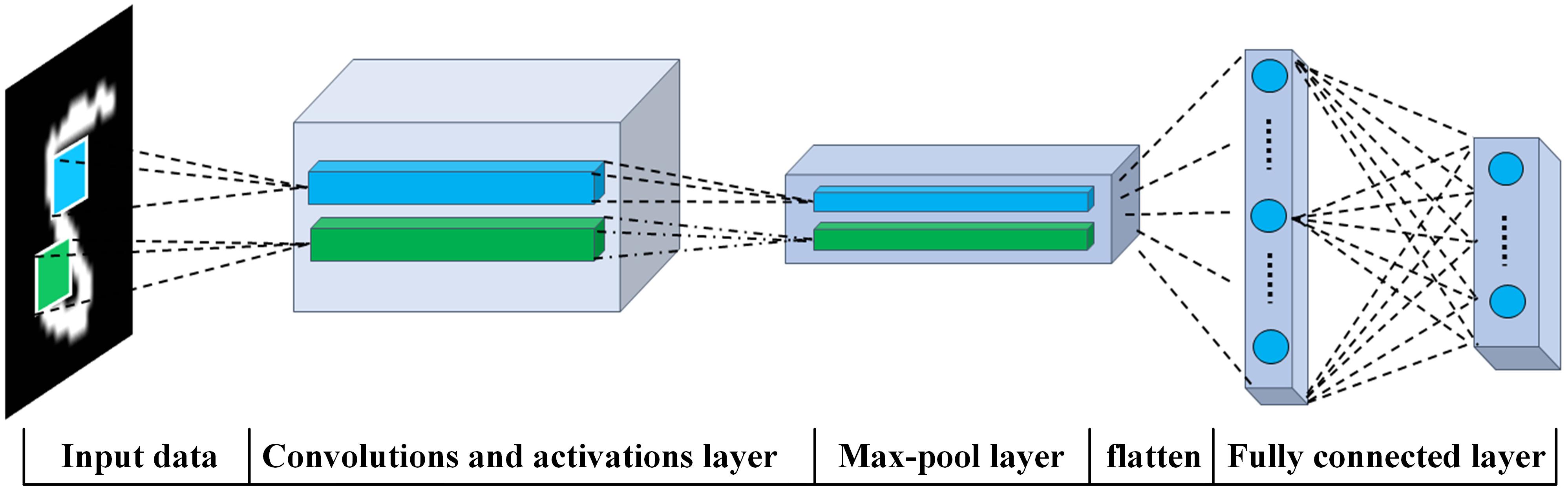
Image classification using CNNs

Image classification assigns a single label to an entire image. CNNs trained on ImageNet (1.2 million images, 1000 classes) now exceed human-level accuracy on that benchmark. The trained network maps raw pixels through convolutional feature extraction to a softmax output layer that produces class probabilities.

Practical applications include facial recognition, medical image diagnosis (e.g., classifying skin lesions or retinal scans), and quality inspection in manufacturing.

Object detection using CNNs

Object detection goes beyond classification: it identifies what objects are in an image and where they are, outputting bounding boxes with class labels. Major architectures fall into two categories:

• Two-stage detectors (R-CNN, Fast R-CNN, Faster R-CNN): First generate region proposals, then classify each proposal. More accurate but slower.
• Single-stage detectors (YOLO, SSD): Predict bounding boxes and classes in one pass through the network. Faster, suitable for real-time applications.

These models train on datasets with bounding box annotations (PASCAL VOC, COCO) and are deployed in autonomous driving, surveillance, and robotics.

Semantic segmentation using CNNs

Semantic segmentation assigns a class label to every pixel in an image, producing a dense prediction map. Architectures typically use an encoder-decoder structure:

• The encoder (often a pre-trained CNN like ResNet) extracts high-level features while reducing spatial resolution.
• The decoder upsamples the features back to the original resolution using transposed convolutions or bilinear interpolation, combined with skip connections from the encoder to preserve fine spatial detail.

Notable architectures include FCN, U-Net (widely used in medical imaging), and DeepLab (which uses atrous/dilated convolutions to capture multi-scale context). Applications range from autonomous driving (road and lane segmentation) to medical imaging (tumor boundary delineation).

Image generation using CNNs

CNNs also power generative models that create new images:

• GANs (Generative Adversarial Networks): A generator CNN creates images while a discriminator CNN tries to distinguish real from generated images. The two networks train adversarially until the generator produces convincing outputs. Applications include synthetic data generation, super-resolution, and style transfer.
• VAEs (Variational Autoencoders): An encoder CNN maps images to a latent distribution, and a decoder CNN reconstructs images from samples of that distribution. VAEs enable smooth interpolation in latent space and controlled generation.

Video analysis using CNNs

Video extends image analysis into the temporal domain. CNN-based approaches include:

• Frame-level CNNs: Apply a 2D CNN to individual frames, then aggregate predictions (e.g., by averaging or voting).
• 3D CNNs: Use 3D convolutional filters (e.g., 3×3×3) that convolve across both spatial and temporal dimensions, directly capturing motion patterns.
• CNN + RNN/LSTM hybrids: A CNN extracts per-frame features, which are then fed into a recurrent network to model temporal dependencies for tasks like action recognition.

Applications include video surveillance, sports analytics, gesture recognition, and content-based video retrieval.

Advanced CNN techniques

Several techniques have been developed to improve CNN performance, efficiency, and robustness beyond the basic architecture.

Transfer learning with CNNs

Transfer learning reuses a model pre-trained on a large dataset (typically ImageNet) for a new task with limited data. Two main strategies:

1. Feature extraction: Freeze the pre-trained convolutional layers and only train a new classifier head on top. Works well when the new task is similar to the original.
2. Fine-tuning: Unfreeze some or all of the pre-trained layers and train the entire network on the new data with a small learning rate. Allows the features to adapt to the new domain.

Transfer learning is especially valuable in signal processing applications where labeled data is scarce (e.g., medical imaging, radar classification). The pre-trained features from early layers (edges, textures) tend to be universal across visual domains.

Data augmentation for CNNs

Data augmentation artificially expands the training set by applying transformations to existing samples. Common augmentations for images include:

• Geometric: rotation, flipping, cropping, scaling, translation
• Photometric: brightness/contrast adjustment, color jittering, adding Gaussian noise
• Advanced: Mixup (blending two images and their labels), CutMix (replacing a patch of one image with a patch from another), random erasing

For 1D signals, augmentations might include time shifting, time stretching, adding noise, or frequency masking. Augmentation reduces overfitting and improves robustness to real-world variability, particularly when training data is limited.

Regularization techniques for CNNs

Regularization prevents overfitting by constraining the model's capacity:

• Dropout: During training, randomly sets a fraction of neuron activations to zero (typically 20-50%). This forces the network to learn redundant representations and acts as an ensemble of sub-networks. At inference time, all neurons are active but outputs are scaled accordingly.
• Weight decay (L2 regularization): Adds a penalty term $\lambda \sum w_i^2$ to the loss function, discouraging large weights and promoting smoother learned functions.
• Batch normalization: Normalizes activations within each mini-batch to have zero mean and unit variance. Stabilizes training, allows higher learning rates, and provides a mild regularization effect.
• Early stopping: Monitors validation loss during training and stops when it begins to increase, preventing the model from memorizing the training data.

These techniques are often combined. A typical modern CNN uses batch normalization in every convolutional block, dropout in fully connected layers, and weight decay in the optimizer.