📡Advanced Signal Processing Unit 1 Review
1.5 Short-time Fourier transform (STFT)
1.5 Short-time Fourier transform (STFT)
Unit & Topic Study Guides
Fourier Analysis and Transforms
Digital Signal Processing Basics
Spectral Estimation and Analysis
Adaptive Filtering & Signal Enhancement
Multirate Processing & Filter Banks
Time-Frequency and Scale Analysis in ASP
Statistical Signal Processing & Estimation
Compressive Sensing & Sparse Signal Processing
Array Processing and Beamforming
Machine Learning in Signal Processing
Signal Processing for Comms and Networks
Biomedical Signal Processing Applications
The Short-time Fourier transform (STFT) solves a core problem with the standard Fourier transform: it can't tell you when different frequencies occur in a signal. By windowing the signal into short segments and transforming each one, the STFT produces a time-frequency representation that tracks how spectral content evolves. This makes it essential for analyzing non-stationary signals in speech processing, music analysis, and biomedical applications.
Definition of STFT
The STFT is a time-frequency analysis technique that computes a localized frequency spectrum at successive time positions along a signal. Rather than transforming the entire signal at once (as the standard Fourier transform does), the STFT multiplies the signal by a short window function centered at a given time, then takes the Fourier transform of that windowed segment. Sliding the window forward and repeating the process builds up a full picture of how frequency content changes over time.
Mathematical representation
The continuous STFT of a signal is defined as:
- is the window function centered at time , selecting a local segment of the signal
- is the frequency variable
- The integral computes the Fourier transform of the product
Note the convention: the window argument is , meaning the window is centered at . Some references write , which is equivalent when the window is symmetric.
The discrete STFT replaces the integral with a summation:
- is the frame (time) index, is the frequency bin index
- is the DFT length (window length, possibly zero-padded)
- is the hop size (the number of samples the window advances between frames)
Continuous vs discrete STFT
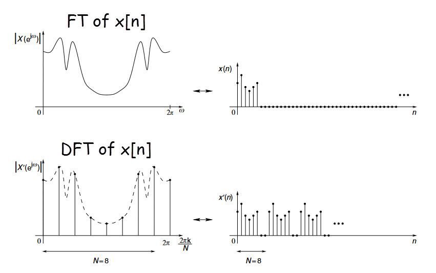
The continuous STFT is a theoretical construct defined for continuous-time signals, yielding a continuous function of both time and frequency. In practice, you work with sampled signals and compute the discrete STFT using the FFT algorithm. The discrete version evaluates the transform at discrete time frames (spaced by the hop size) and discrete frequency bins (spaced by , where is the sampling rate).
STFT vs Fourier transform
Both the STFT and the standard Fourier transform decompose a signal into sinusoidal components using complex exponential basis functions, and both produce magnitude and phase spectra.
Similarities in frequency analysis
- Both represent the signal in terms of frequency components
- Both use the same complex exponential basis
- The output of both includes magnitude (how strong each frequency is) and phase (the timing alignment of each component)
Differences in time-frequency resolution
The standard Fourier transform integrates over the entire signal, producing a single global spectrum with no time information. You know what frequencies are present, but not when they occur.
The STFT introduces time localization by analyzing short windowed segments. You get a spectrum for each time position, so you can track frequency changes. The cost is reduced frequency resolution: a shorter analysis window means fewer cycles of a sinusoid fit inside it, which broadens the spectral peaks.
Time-frequency resolution tradeoff
The STFT faces a fundamental tradeoff between time and frequency resolution, rooted in the Heisenberg-Gabor uncertainty principle.
Uncertainty principle
The uncertainty principle places a lower bound on the product of time resolution and frequency resolution :
You cannot make both arbitrarily small simultaneously. Narrowing the window (better time resolution) necessarily widens the frequency uncertainty, and vice versa. This is not a limitation of the algorithm; it's a fundamental property of Fourier analysis.
Window size impact
- Short window: captures rapid temporal changes (good time resolution), but each segment contains few oscillation cycles, so closely spaced frequencies blur together (poor frequency resolution)
- Long window: contains many oscillation cycles, allowing fine frequency discrimination (good frequency resolution), but temporal events get smeared across the window duration (poor time resolution)
Choosing the window length is always application-dependent. For a signal with fast transients (like percussive sounds), you'd favor a shorter window. For a signal with closely spaced tones (like two nearby musical notes), a longer window helps separate them.
Overlap between windows
Overlapping consecutive windows smooths the time-frequency representation and prevents events from being split awkwardly between frames. Typical overlap values are 50% to 75% of the window length. Higher overlap gives denser time sampling (more frames per second) at the cost of increased computation, but it does not improve the underlying time-frequency resolution set by the window size.
STFT parameters
Three interrelated parameters control the STFT's behavior: the window function, the window length, and the hop size.
Window function types
The window function shapes each segment before the FFT. Different windows trade off between mainlobe width (frequency resolution) and sidelobe level (spectral leakage suppression):
| Window | Mainlobe Width | Sidelobe Level | Use Case |
|---|---|---|---|
| Rectangular | Narrowest | Highest (-13 dB) | Maximum frequency resolution, but severe leakage |
| Hann | Moderate | Low (-31 dB) | General-purpose; good leakage suppression |
| Hamming | Moderate | Lower (-43 dB) | Similar to Hann with better near-sidelobe suppression |
| Gaussian | Depends on | Very low | Achieves the theoretical minimum uncertainty product |
| Blackman-Harris | Wide | Very low (-92 dB) | When sidelobe suppression is critical |
The Hann window is the most common default choice. The Gaussian window is notable because it achieves the minimum product, making it optimal in the uncertainty-principle sense.
Window length selection
The window length directly sets the time-frequency resolution balance:
- Time resolution seconds
- Frequency resolution Hz
For example, at Hz with : time resolution is about 32 ms and frequency resolution is about 31.25 Hz. Doubling to 1024 halves the frequency resolution to ~15.6 Hz but doubles the time resolution to ~64 ms.
Hop size determination
The hop size is the number of samples between successive window positions. It controls how densely you sample the time axis:
- Hop size = window length (no overlap): fastest computation, but temporal gaps may miss events
- Hop size = window length / 2 (50% overlap): standard choice balancing density and cost
- Hop size = window length / 4 (75% overlap): smoother representation, needed for some reconstruction algorithms
For perfect reconstruction (inverting the STFT back to a time-domain signal), the hop size and window must satisfy the constant overlap-add (COLA) constraint.
STFT computation
Computing the STFT follows a straightforward sliding-window procedure.
Sliding window approach
- Place the window function at the beginning of the signal (centered at frame )
- Multiply the signal samples within the window by the window function values, producing a windowed segment
- Advance the window by the hop size samples
- Repeat steps 2-3 until the window has traversed the entire signal
FFT of windowed signal
For each windowed segment:
- (Optional) Zero-pad the segment to a length that is a power of 2, which speeds up the FFT and interpolates the frequency axis for smoother spectra
- Compute the FFT of the windowed (and possibly zero-padded) segment
- Store the resulting complex-valued spectrum as one column of the STFT matrix
The output is a 2D complex matrix with time frames along one axis and frequency bins along the other.
Spectrogram representation
The spectrogram is the squared magnitude of the STFT:
It's displayed as a 2D image with time on the horizontal axis, frequency on the vertical axis, and color (or intensity) encoding the power at each time-frequency point. Spectrograms are often plotted on a logarithmic (dB) scale to make quiet components visible alongside loud ones.
Interpreting STFT results
Time-frequency plane
Each point in the STFT matrix corresponds to a specific time frame and frequency bin. The magnitude at that point tells you how much energy the signal has at that frequency during that time window. Reading across a row (fixed frequency) shows how that frequency's energy evolves over time. Reading down a column (fixed time) gives the instantaneous spectrum at that moment.
Magnitude vs phase information
The STFT coefficients are complex-valued: .
- Magnitude tells you the strength of each frequency component at each time. This is what the spectrogram displays, and it's what most analysis tasks rely on.
- Phase encodes the temporal alignment of each component. Phase is critical for signal reconstruction (inverse STFT) and for techniques like the phase vocoder used in time-stretching and pitch-shifting audio.
Identifying signal components
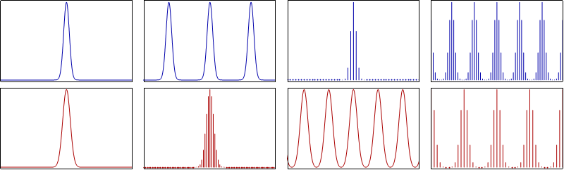
Different signal features produce characteristic patterns in the spectrogram:
- Stationary tones appear as horizontal bands at constant frequency
- Frequency sweeps (chirps) appear as diagonal or curved traces
- Transients (clicks, onsets) appear as vertical lines spanning many frequencies at a single time instant
- Harmonics of a periodic signal appear as a stack of evenly spaced horizontal bands
- Broadband noise fills a wide frequency range with relatively uniform energy
Applications of STFT
Speech processing
- Speech recognition: STFT-derived features (like mel-frequency spectrograms) serve as input to recognition models. The time-frequency representation captures formant transitions and phoneme boundaries.
- Speech enhancement: Noise components can be identified and suppressed in the time-frequency domain (e.g., spectral subtraction), then the cleaned signal is reconstructed via inverse STFT.
- Voice activity detection: Speech segments show structured harmonic patterns in the spectrogram, while silence or noise does not, making it straightforward to detect when someone is speaking.
Music analysis
- Pitch estimation: The fundamental frequency and its harmonics appear as distinct peaks in each STFT frame, enabling pitch tracking over time.
- Onset detection: Musical note onsets produce transient broadband energy bursts that are visible as vertical features in the spectrogram.
- Music transcription: Combining pitch estimation and onset detection across time frames allows conversion of audio into symbolic notation (e.g., MIDI).
Biomedical signal processing
- EEG analysis: Brain rhythms (alpha, beta, theta, delta bands) occupy specific frequency ranges. The STFT reveals how these rhythms change during different cognitive states or in response to stimuli.
- ECG analysis: Time-frequency representations help detect arrhythmias and other cardiac events that involve transient changes in the heart's electrical activity.
- EMG analysis: Muscle fatigue manifests as a shift in the median frequency of the EMG power spectrum over time, which the STFT can track.
Limitations of STFT
Fixed time-frequency resolution
The most significant limitation: once you choose a window length, the time-frequency resolution is locked for the entire analysis. A signal that contains both fast transients and closely spaced steady tones cannot be optimally analyzed with a single fixed window. This is the primary motivation for multi-resolution methods like the wavelet transform.
Spectral leakage
When a signal's frequency components don't fall exactly on the DFT's discrete frequency bins, their energy "leaks" into neighboring bins. This creates artificial sidelobes in the spectrum. Window functions reduce leakage by tapering the segment edges to zero, but they also widen the mainlobe, reducing frequency resolution. There's no window that eliminates leakage entirely without sacrificing resolution.
Boundary effects
At the beginning and end of the signal, the window extends beyond the available data. The standard assumption is that the signal is zero outside its duration, but this introduces discontinuities that distort the spectrum in those edge frames. Common mitigations include zero-padding, reflecting the signal at its boundaries, or simply discarding the edge frames from the analysis.
Advanced STFT techniques
Multi-resolution analysis
Multi-resolution approaches use different window lengths for different frequency bands. Low frequencies (which need fine frequency resolution) get long windows, while high frequencies (which need fine time resolution) get short windows. The wavelet transform implements this naturally through its dyadic scaling structure. Multi-resolution STFT variants achieve similar effects by computing multiple STFTs with different window sizes and combining the results.
Adaptive window sizes
Rather than fixing the window length globally or by frequency band, adaptive methods choose the window size locally based on the signal's characteristics at each time instant. For example, if the signal is locally stationary, a longer window is selected for better frequency resolution; if a transient is detected, the window shortens to capture it precisely. These methods add computational complexity but can significantly improve the representation for signals with diverse time-frequency behavior.
Synchrosqueezing transform
Synchrosqueezing is a post-processing step applied to the STFT that sharpens the time-frequency representation. It works by:
- Computing the standard STFT
- Estimating the instantaneous frequency at each time-frequency point from the phase derivative:
- Reassigning each STFT coefficient from its original frequency bin to the bin corresponding to its estimated instantaneous frequency
This concentrates energy more tightly around the true frequency trajectories, producing a crisper spectrogram. Unlike the standard STFT, the synchrosqueezed representation is invertible, meaning you can reconstruct the signal from it. It's particularly effective for signals composed of well-separated amplitude- and frequency-modulated components.