📡Advanced Signal Processing Unit 2 Review
2.7 Discrete Fourier transform (DFT)
2.7 Discrete Fourier transform (DFT)
Unit & Topic Study Guides
Fourier Analysis and Transforms
Digital Signal Processing Basics
Spectral Estimation and Analysis
Adaptive Filtering & Signal Enhancement
Multirate Processing & Filter Banks
Time-Frequency and Scale Analysis in ASP
Statistical Signal Processing & Estimation
Compressive Sensing & Sparse Signal Processing
Array Processing and Beamforming
Machine Learning in Signal Processing
Signal Processing for Comms and Networks
Biomedical Signal Processing Applications
Definition of DFT
The Discrete Fourier Transform (DFT) converts a finite sequence of equally-spaced samples into a same-length sequence of frequency-domain coefficients. It's the practical, computable version of the Discrete-Time Fourier Transform (DTFT), which produces a continuous frequency spectrum you can't actually store or compute digitally.
The DFT is central to nearly every frequency-domain operation in DSP: spectral analysis, filtering, compression, and resampling all rely on it.
Mathematical formulation
The DFT of a length- sequence is defined as:
The inverse DFT (IDFT) recovers the time-domain sequence:
Together these form a transform pair. Each DFT bin represents the signal's content at frequency , where is the sampling rate. The complex exponential acts as the analysis basis function, correlating the input with a sinusoid at that frequency.
Relationship to Fourier series
The DFT can be understood as a sampled version of the Fourier series. For a periodic sequence with period , the DFT coefficients are exactly the Fourier series coefficients (up to scaling).
This connection matters because the DFT inherently treats its input as one period of a periodic signal. Whether or not your original signal is actually periodic, the DFT behaves as though it repeats every samples.
Periodic vs aperiodic signals
Because the DFT assumes periodicity, applying it to an aperiodic signal means the signal is implicitly extended by repeating the -sample block end-to-end. If the first and last samples don't match up smoothly, this creates artificial discontinuities at the block boundaries.
These discontinuities produce artifacts in the frequency domain:
- Spectral leakage: energy from a single frequency spreads across multiple DFT bins
- Picket-fence effect: true frequency components falling between DFT bins get misrepresented
Both can be reduced using windowing (to taper the signal edges) and zero-padding (to interpolate finer frequency bins).
Properties of DFT
The DFT has several algebraic properties that make it useful for signal manipulation. These properties let you predict how time-domain operations translate to the frequency domain and vice versa.
Linearity
The DFT is linear, satisfying both additivity and homogeneity:
- Additivity:
- Homogeneity:
This means you can analyze composite signals by computing the DFT of each component separately and summing the results.
Periodicity in time and frequency
Both the input sequence and the DFT output are implicitly periodic with period :
- Time domain: for all
- Frequency domain: for all
This is why all index arithmetic in DFT-based operations is modulo . Circular (not linear) operations are the natural domain of the DFT.
Symmetry properties
For a real-valued input sequence , the DFT exhibits conjugate symmetry:
- for
- The real part is even:
- The imaginary part is odd:
This means only the first bins carry unique information for real signals. You can exploit this to halve storage and computation.
Convolution vs multiplication
The DFT converts between convolution and multiplication:
-
Circular convolution in time corresponds to pointwise multiplication in frequency:
-
Pointwise multiplication in time corresponds to circular convolution in frequency (scaled by ):
Note the distinction: this is circular convolution, not linear convolution. To use the DFT for linear convolution (e.g., FIR filtering), you need to zero-pad both sequences to length before transforming, so the circular result matches the linear one.
Computation of DFT
Direct computation
Evaluating the DFT definition directly for each of the output bins requires:
- complex multiplications per bin bins = complex multiplications
- complex additions
The overall complexity is . For , that's operations, which is impractical for real-time processing.
Fast Fourier Transform (FFT) algorithms
FFT algorithms reduce the complexity to by exploiting the symmetry and periodicity of the complex exponential basis functions. The core idea is divide-and-conquer: decompose a large DFT into combinations of smaller DFTs.
For , the FFT requires roughly operations instead of , a speedup of about 50,000x.
Radix-2 FFT
The radix-2 FFT applies when . It works by:
- Splitting the -point sequence into two -point subsequences (even-indexed and odd-indexed samples)
- Computing the -point DFT of each subsequence recursively
- Combining the two half-length DFTs using the butterfly operation, which multiplies the odd-indexed DFT by twiddle factors and adds/subtracts from the even-indexed DFT
This recursion continues until you reach 2-point DFTs, which are trivial. The result is complexity.
Cooley-Tukey algorithm
The Cooley-Tukey algorithm generalizes the radix-2 approach to any composite length . It decomposes the -point DFT into DFTs of size (or vice versa), with twiddle factor multiplications between stages.
- Radix-2 is the special case where ,
- Mixed-radix variants handle lengths like , which is why many FFT libraries (e.g., FFTW) perform well for "smooth" values of , not just powers of 2
- For prime-length DFTs, algorithms like Bluestein's or Rader's are used instead
Sampling and aliasing
Sampling and aliasing are prerequisites for understanding what the DFT can and cannot tell you about a signal. The DFT operates on sampled data, so the quality of that sampling directly determines the validity of the frequency-domain results.
Nyquist-Shannon sampling theorem
A continuous-time bandlimited signal can be perfectly reconstructed from its samples if the sampling frequency satisfies:
where is the highest frequency present in the signal. The threshold is called the Nyquist rate.
If you sample a 10 kHz bandwidth signal, you need kHz. CD audio uses 44.1 kHz to capture the audible range up to about 20 kHz, with some margin for the anti-aliasing filter's transition band.
Aliasing in time and frequency domains
When , frequency components above fold back into the range and become indistinguishable from lower-frequency components. This is aliasing.
- Time domain: high-frequency content appears as spurious low-frequency oscillations in the sampled signal
- Frequency domain: spectral replicas (centered at multiples of ) overlap, corrupting the baseband spectrum
Once aliasing has occurred during sampling, it cannot be undone. The corrupted frequency components are permanently mixed with the true signal content.
Anti-aliasing filters
Anti-aliasing filters are analog low-pass filters applied before the ADC to remove frequency content above :
- Ideal filter: brick-wall cutoff at (not physically realizable)
- Practical filters: have a transition band between the passband edge and the stopband, requiring some oversampling margin
Common filter types with different design trade-offs:
- Butterworth: maximally flat passband, gentle rolloff
- Chebyshev Type I: steeper rolloff, passband ripple
- Elliptic (Cauer): steepest rolloff for a given order, but ripple in both passband and stopband
The choice depends on how much passband distortion is acceptable versus how sharp the cutoff needs to be.
Applications of DFT

Spectral analysis
Spectral analysis uses the DFT to decompose a signal into its frequency components. The magnitude reveals which frequencies are present and how strong they are; the phase captures timing relationships.
Practical applications include:
- Audio processing: pitch detection, musical note identification, equalization. A 1024-point FFT at 44.1 kHz gives frequency resolution of about 43 Hz per bin.
- Vibration analysis: detecting bearing faults or imbalance in rotating machinery by identifying characteristic fault frequencies
- Power systems: monitoring harmonic distortion (e.g., identifying 3rd, 5th, 7th harmonics of 50/60 Hz mains frequency)
Filtering in frequency domain
Frequency-domain filtering exploits the circular convolution theorem to implement filtering as pointwise multiplication:
- Compute the DFT of the input signal and the filter impulse response (both zero-padded to avoid circular convolution artifacts)
- Multiply elementwise:
- Compute the IDFT of to get the filtered output
This approach is more efficient than direct time-domain convolution when the filter length is large. The crossover point is roughly when , though in practice overlap-add or overlap-save methods are used for continuous (block-by-block) processing.
Signal compression
The DFT and its variants are used in transform coding, where signals are represented in the frequency domain and less perceptually important coefficients are discarded or coarsely quantized.
- Audio compression: Standards like MP3 and AAC use the Modified Discrete Cosine Transform (MDCT), which is closely related to the DFT. The signal is divided into overlapping blocks, transformed, and the coefficients are quantized according to a psychoacoustic model.
- Subband coding: The signal is split into frequency bands that are encoded independently. Different bit allocations per band allow efficient compression.
Note that image compression standards like JPEG use the DCT (a real-valued relative of the DFT), while JPEG 2000 uses wavelets, which are a different transform family altogether.
Interpolation and resampling
The DFT provides a clean framework for changing the sampling rate of a signal:
- Upsampling (increasing rate): Zero-pad the DFT spectrum symmetrically (insert zeros in the high-frequency region), then take the IDFT. The result has more samples representing the same signal.
- Downsampling (decreasing rate): Truncate the DFT spectrum to keep only the low-frequency bins (after verifying no aliasing), then take the IDFT.
- Arbitrary resampling: Combine upsampling, low-pass filtering, and downsampling. The DFT-based approach handles this efficiently in the frequency domain.
The key insight is that zero-padding in the frequency domain produces sinc interpolation in the time domain, which is the theoretically optimal interpolation for bandlimited signals.
Limitations of DFT
Finite length signals
The DFT operates on exactly samples and implicitly treats them as one period of a periodic signal. If the signal doesn't naturally repeat every samples, the periodic extension creates discontinuities at the block boundaries.
These boundary discontinuities are the root cause of both spectral leakage and reduced frequency resolution. Window functions (Hann, Hamming, Blackman, Kaiser, etc.) taper the signal toward zero at the edges, smoothing out the discontinuities at the cost of slightly reduced frequency resolution in the main lobe.
Spectral leakage
Spectral leakage occurs when a signal's frequency components don't land exactly on DFT bin centers. The energy from that component "leaks" into neighboring bins through the sidelobes of the window function's frequency response.
Two factors drive leakage:
- Finite observation length: truncating the signal is equivalent to multiplying by a rectangular window, whose transform (a sinc function) has significant sidelobes
- Frequency mismatch: if a sinusoid at frequency falls between bins and , its energy spreads across many bins
Window functions trade main-lobe width (frequency resolution) for sidelobe suppression (leakage reduction). A rectangular window has the narrowest main lobe but the worst sidelobes. A Blackman window has very low sidelobes but a wider main lobe.
Picket-fence effect
The DFT only evaluates the spectrum at discrete frequencies spaced apart. You're viewing the true continuous spectrum through a "picket fence" and can miss what falls between the slats.
For example, with Hz and , the bin spacing is 10 Hz. A tone at 105 Hz falls exactly between bins 10 (100 Hz) and 11 (110 Hz), so its energy splits between them and neither bin shows the true amplitude.
Mitigation strategies:
- Zero-padding: appending zeros increases and reduces , giving finer interpolation of the spectrum
- Parabolic or sinc interpolation: estimating the true peak location from adjacent bin values
Zero-padding techniques
Zero-padding appends zeros to the end of the signal before computing the DFT. If you have data samples and pad to length , the DFT bin spacing becomes instead of .
What zero-padding does:
- Interpolates between the original frequency bins, giving a smoother-looking spectrum
- Makes it easier to identify peaks that fall between original bins
- Enables use of radix-2 FFT by padding to the next power of 2
What zero-padding does not do:
- It does not add new spectral information. The underlying frequency resolution is still determined by the original signal length .
- It does not reduce spectral leakage. Only windowing addresses that.
A common practice is to pad to at least or for visualization, and to the next power of 2 for computational efficiency.
DFT vs other transforms
DFT vs Discrete-Time Fourier Transform (DTFT)
The DTFT produces a continuous, periodic function of frequency for a discrete-time sequence:
Key differences:
| DFT | DTFT | |
|---|---|---|
| Input length | Finite ( samples) | Can be infinite |
| Frequency variable | Discrete ( bins) | Continuous () |
| Computable | Yes, directly | No (requires evaluation at infinite points) |
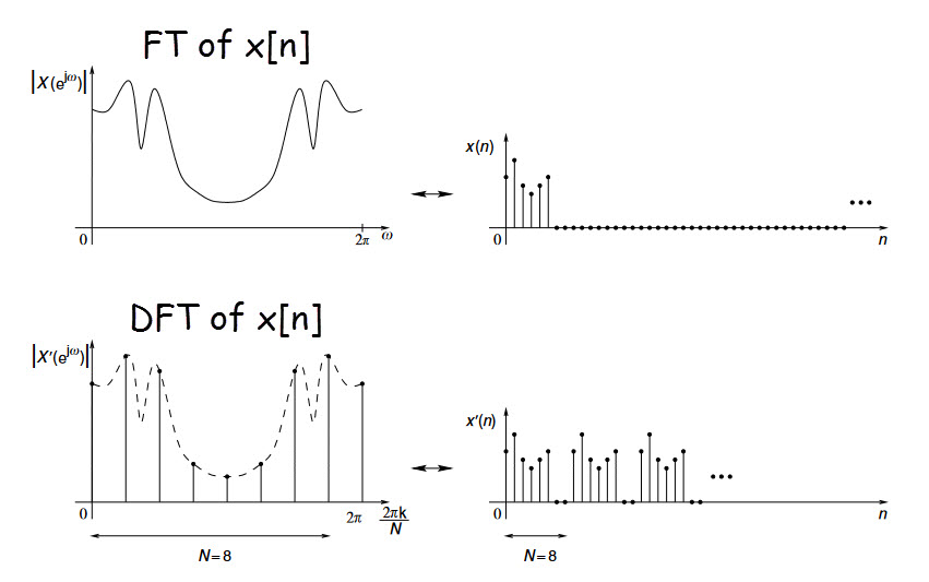
| Relationship | Samples of the DTFT at | Continuous envelope that the DFT samples |
The DFT is essentially equally-spaced samples of the DTFT of the windowed (finite-length) signal. This is why zero-padding the DFT gives you more samples of the same underlying DTFT, not a higher-resolution DTFT.