7.4 Maximum likelihood estimation (MLE)

Basics of Maximum Likelihood Estimation

Maximum likelihood estimation (MLE) is a method for estimating the parameters of a probability distribution by finding the parameter values that make the observed data most probable. In signal processing, MLE is the go-to framework for extracting unknown quantities from noisy observations, whether you're estimating a carrier frequency, detecting a radar pulse, or classifying a modulation scheme.

The core idea: given a parametric model for your data, construct a function that scores how "likely" each candidate parameter value is, then pick the value that scores highest.

Definition

Given observed data $\mathbf{x} = [x_1, x_2, \dots, x_N]$ and a parametric family of distributions $p(\mathbf{x};\boldsymbol{\theta})$, the MLE is defined as:

$\hat{\boldsymbol{\theta}}_{\text{ML}} = \arg\max_{\boldsymbol{\theta}} \; p(\mathbf{x};\boldsymbol{\theta})$

The function $L(\boldsymbol{\theta}) = p(\mathbf{x};\boldsymbol{\theta})$, viewed as a function of $\boldsymbol{\theta}$ with $\mathbf{x}$ fixed, is the likelihood function. Note the subtle but important shift: the density is the same mathematical expression, but now the data are fixed and the parameters vary.

Principles

MLE rests on a straightforward principle: the parameter value that would have generated the observed data with highest probability is the best estimate. To carry this out:

1. Write down the joint density (or mass function) of the data given the parameters.
2. Treat that expression as a function of the parameters alone.
3. Find the parameters that maximize it.

In practice, you almost always work with the log-likelihood instead (covered below), because products turn into sums and the calculus becomes much cleaner.

Assumptions

• The observations are independently and identically distributed (i.i.d.) according to the assumed model. This lets you write the joint likelihood as a product of marginals.
• The parametric form of the distribution is known; only the parameter values are unknown.
• The model is correctly specified, meaning the true data-generating process actually belongs to the assumed family. When this assumption breaks, MLE can still work reasonably well, but its optimality guarantees weaken.

MLE for Parameter Estimation

Single-Parameter Case

For a single unknown parameter $\theta$, the procedure is direct. Suppose you observe $N$ i.i.d. samples from an exponential distribution with unknown rate $\lambda$. The likelihood is:

$L(\lambda) = \prod_{n=1}^{N} \lambda \, e^{-\lambda x_n} = \lambda^N \, e^{-\lambda \sum x_n}$

Taking the log, differentiating with respect to $\lambda$, and setting the result to zero gives $\hat{\lambda}_{\text{ML}} = N / \sum_{n=1}^{N} x_n$, which is just the reciprocal of the sample mean.

Multiple-Parameter Case

When the model has a parameter vector $\boldsymbol{\theta} = [\theta_1, \theta_2, \dots, \theta_p]^T$, you maximize the likelihood jointly over all parameters. This means setting the gradient of the log-likelihood to zero:

$\nabla_{\boldsymbol{\theta}} \, \ell(\boldsymbol{\theta}) = \mathbf{0}$

This yields a system of $p$ equations (the score equations) that must be solved simultaneously. For a Gaussian model with unknown mean $\mu$ and variance $\sigma^2$, for instance, you get the familiar sample mean and sample variance as the joint MLEs.

Properties of MLE Estimators

Three properties make MLE especially attractive for signal processing:

• Consistency: $\hat{\boldsymbol{\theta}}_{\text{ML}} \xrightarrow{p} \boldsymbol{\theta}_0$ as $N \to \infty$. With enough data, the estimate converges to the true value.
• Asymptotic efficiency: For large $N$, the MLE achieves the Cramér-Rao lower bound (CRLB). No unbiased estimator can have lower variance in the asymptotic regime.
• Invariance: If $\hat{\theta}_{\text{ML}}$ is the MLE of $\theta$, then $g(\hat{\theta}_{\text{ML}})$ is the MLE of $g(\theta)$ for any function $g$. This is useful when you estimate one parameterization but need another (e.g., estimating variance but reporting standard deviation).

A common pitfall: MLE is not necessarily unbiased for finite samples. The classic example is the Gaussian variance estimate, which has a bias factor of $(N-1)/N$.

Derivation of MLE

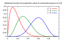
Likelihood Function

For i.i.d. observations $x_1, \dots, x_N$, the likelihood factors as:

$L(\boldsymbol{\theta}) = \prod_{n=1}^{N} p(x_n; \boldsymbol{\theta})$

This product form is a direct consequence of the independence assumption. Each factor scores how well the candidate $\boldsymbol{\theta}$ explains a single observation.

Log-Likelihood Function

Taking the natural logarithm converts the product into a sum:

$\ell(\boldsymbol{\theta}) = \ln L(\boldsymbol{\theta}) = \sum_{n=1}^{N} \ln p(x_n; \boldsymbol{\theta})$

Because $\ln(\cdot)$ is strictly monotonically increasing, maximizing $\ell$ is equivalent to maximizing $L$. The log-likelihood is almost always preferred because:

• Sums are numerically more stable than products of many small probabilities.
• Exponential-family distributions yield log-likelihoods that are polynomial in the parameters, making differentiation straightforward.

Solving the MLE Equations

Step-by-step procedure for finding the MLE:

1. Write the log-likelihood $\ell(\boldsymbol{\theta})$.
2. Compute the partial derivatives $\partial \ell / \partial \theta_i$ for each parameter.
3. Set all partial derivatives to zero (the score equations).
4. Solve the resulting system of equations for $\boldsymbol{\theta}$.
5. Verify that the solution is a maximum (not a minimum or saddle point) by checking the second-order conditions: the Hessian matrix of $\ell$ should be negative definite at the solution.

When the score equations have a closed-form solution, you're done analytically. When they don't, you turn to numerical methods (see below).

MLE in Signal Processing Applications

Signal Detection

In binary hypothesis testing, you observe $\mathbf{x}$ and decide between $H_0$ (noise only) and $H_1$ (signal plus noise). The generalized likelihood ratio test (GLRT) uses MLE when the signal parameters are unknown:

$\Lambda(\mathbf{x}) = \frac{\max_{\boldsymbol{\theta}} \; p(\mathbf{x}; \boldsymbol{\theta}, H_1)}{p(\mathbf{x}; H_0)} \underset{H_0}{\overset{H_1}{\gtrless}} \gamma$

You first compute the MLE of the unknown parameters under $H_1$, plug them back into the likelihood, and compare the ratio to a threshold $\gamma$. This is the standard approach when a pure Neyman-Pearson test isn't available because of unknown parameters.

Signal Parameter Estimation

Estimating parameters like amplitude, frequency, or time delay from noisy observations is a natural MLE problem. For a sinusoid in additive white Gaussian noise (AWGN):

$x_n = A\cos(2\pi f_0 n + \phi) + w_n, \quad w_n \sim \mathcal{N}(0, \sigma^2)$

The MLE of frequency $f_0$ reduces to finding the peak of the periodogram (the squared magnitude of the DFT). The MLE of amplitude and phase then follow in closed form once $f_0$ is fixed. This is a good example of how MLE connects to classical spectral analysis.

Signal Classification

For classifying a received signal into one of $M$ classes, MLE assigns the observation to the class with the highest likelihood:

$\hat{c} = \arg\max_{c \in \{1, \dots, M\}} \; p(\mathbf{x}; \hat{\boldsymbol{\theta}}_c, c)$

This is equivalent to the maximum likelihood classifier. When class priors are equal, it coincides with the MAP (maximum a posteriori) classifier.

Advantages and Limitations of MLE

Advantages

• Asymptotic optimality: Achieves the CRLB for large sample sizes, so you can't do better in terms of variance.
• Invariance: Reparameterize freely without re-deriving the estimator.
• Unified framework: The same methodology applies whether you're estimating one parameter or fifty, for Gaussian or non-Gaussian models.

Limitations

• Model dependence: If the assumed distribution is wrong, the MLE may be biased or inconsistent. There's no free lunch.
• Sensitivity to outliers: Because MLE maximizes the likelihood of all observations, a few extreme outliers can pull the estimate significantly.
• No closed-form solution in many cases: Complex signal models often require iterative numerical optimization, which introduces concerns about convergence and computational cost.
• Finite-sample bias: The asymptotic guarantees don't always hold for small $N$. For short data records (common in radar or communications), MLE performance can fall well short of the CRLB.

MLE vs. Other Estimation Methods

In signal processing, Bayesian methods and MLE are often used together: MLE provides the likelihood model, and Bayesian inference adds prior knowledge to improve performance in low-SNR or data-starved scenarios.

Numerical Methods for MLE

When the score equations can't be solved in closed form, you need iterative algorithms.

Newton-Raphson Method

Newton-Raphson uses both the gradient and curvature of the log-likelihood to take intelligent steps toward the maximum:

$\boldsymbol{\theta}^{(k+1)} = \boldsymbol{\theta}^{(k)} - \left[\mathbf{H}\left(\boldsymbol{\theta}^{(k)}\right)\right]^{-1} \nabla \ell\left(\boldsymbol{\theta}^{(k)}\right)$

where $\mathbf{H}$ is the Hessian matrix of second partial derivatives. This converges quadratically near the solution, but it requires computing and inverting the Hessian at each step, which can be expensive for high-dimensional problems.

A common variant replaces the Hessian with its expected value (the negative Fisher information matrix), giving the Fisher scoring algorithm. This is often more stable because the Fisher information matrix is guaranteed to be positive semi-definite.

Expectation-Maximization (EM) Algorithm

The EM algorithm handles MLE when the data are incomplete or when latent variables are present (e.g., mixture models, hidden Markov models). It iterates between two steps:

1. E-step: Compute the expected log-likelihood of the complete data, using the current parameter estimates and the observed data: $Q(\boldsymbol{\theta} | \boldsymbol{\theta}^{(k)}) = E\left[\ln p(\mathbf{x}, \mathbf{z}; \boldsymbol{\theta}) \mid \mathbf{x}, \boldsymbol{\theta}^{(k)}\right]$ where $\mathbf{z}$ represents the latent/missing data.

2. M-step: Maximize $Q$ with respect to $\boldsymbol{\theta}$: $\boldsymbol{\theta}^{(k+1)} = \arg\max_{\boldsymbol{\theta}} \; Q(\boldsymbol{\theta} | \boldsymbol{\theta}^{(k)})$

EM is guaranteed to increase the likelihood at each iteration (or leave it unchanged), so it never diverges. The trade-off is that convergence can be slow, and it only guarantees convergence to a local maximum.

Gradient-Based Optimization

Gradient ascent updates parameters in the direction of steepest increase:

$\boldsymbol{\theta}^{(k+1)} = \boldsymbol{\theta}^{(k)} + \mu \, \nabla \ell\left(\boldsymbol{\theta}^{(k)}\right)$

where $\mu$ is the step size (learning rate). This is simpler than Newton-Raphson since it avoids the Hessian, but convergence is only linear and can be sensitive to the choice of $\mu$.

For large-scale problems (large $N$ or streaming data), stochastic gradient ascent approximates the full gradient using a subset of the data at each step, trading per-iteration accuracy for computational speed.

Advanced Topics in MLE

Constrained MLE

When parameters must satisfy constraints (e.g., a covariance matrix must be positive definite, or probabilities must sum to one), you solve a constrained optimization problem. Standard approaches include:

• Lagrange multipliers for equality constraints
• Barrier/interior-point methods for inequality constraints
• Reparameterization to eliminate constraints (e.g., optimizing over the Cholesky factor of a covariance matrix instead of the matrix itself)

MLE with Missing Data

Missing data arise frequently in sensor networks (dropped packets), array processing (failed elements), and spectral analysis (non-uniform sampling). The EM algorithm is the standard tool here, treating the missing observations as latent variables and iterating between imputation (E-step) and estimation (M-step).

MLE for Non-Linear Models

Many signal processing models are non-linear in the parameters (e.g., estimating time delays, Doppler shifts, or directions of arrival). The log-likelihood surface for these problems is often multimodal, so:

• Global search methods (grid search, genetic algorithms) may be needed to find a good initialization.
• Local refinement via Gauss-Newton or Levenberg-Marquardt then converges to the nearest peak.
• The computational cost scales with the dimensionality of the parameter space and the number of local optima.

MAP Estimation and Its Relation to MLE

Maximum a posteriori (MAP) estimation incorporates prior information through Bayes' theorem:

$\hat{\boldsymbol{\theta}}_{\text{MAP}} = \arg\max_{\boldsymbol{\theta}} \; p(\boldsymbol{\theta} | \mathbf{x}) = \arg\max_{\boldsymbol{\theta}} \; \left[ \ln p(\mathbf{x}; \boldsymbol{\theta}) + \ln p(\boldsymbol{\theta}) \right]$

MAP reduces to MLE when the prior $p(\boldsymbol{\theta})$ is uniform (non-informative). In signal processing, MAP is useful when you have physical constraints or prior measurements that should influence the estimate. The prior acts as a regularizer, which can prevent overfitting and improve performance at low SNR.

Practical Considerations

Choice of Initial Values

Iterative MLE algorithms are sensitive to initialization. Strategies that work well in practice:

• Use method of moments estimates as a starting point.
• Perform a coarse grid search over the parameter space to identify the region of the global maximum.
• Run the algorithm from multiple random initializations and keep the solution with the highest log-likelihood.
• Exploit problem structure: for frequency estimation, the FFT peak gives a good initial frequency; for mixture models, k-means clustering provides initial component assignments.

Assessing Convergence

Monitor convergence by tracking the log-likelihood value across iterations. Common stopping criteria:

• The change in log-likelihood falls below a threshold: $|\ell^{(k+1)} - \ell^{(k)}| < \epsilon$
• The change in parameter estimates falls below a threshold: $\|\boldsymbol{\theta}^{(k+1)} - \boldsymbol{\theta}^{(k)}\| < \delta$
• A maximum number of iterations is reached (as a safety net)

If the log-likelihood decreases at any iteration (for Newton-Raphson or gradient methods), the step size is too large or the Hessian approximation is poor.

Computational Complexity

The cost per iteration depends on the algorithm and model:

• Newton-Raphson: $O(p^3)$ per iteration due to Hessian inversion, where $p$ is the number of parameters.
• Gradient ascent: $O(Np)$ per iteration for computing the gradient over $N$ data points.
• EM: Depends heavily on the model; the E-step can be the bottleneck for complex latent-variable models.

For real-time signal processing, computational budget often dictates the choice of algorithm. Approximate or online MLE methods trade statistical efficiency for speed.

Robustness

MLE estimators can break down when the model assumptions are violated. To guard against this:

• Use robust alternatives like M-estimators, which replace the log-likelihood with a less outlier-sensitive loss function (e.g., Huber's loss).
• Apply goodness-of-fit tests (Kolmogorov-Smirnov, chi-squared) to check whether the assumed distribution fits the data.
• Consider model selection criteria (AIC, BIC) to choose among competing models, balancing fit quality against model complexity.