7.1 Feedback control architectures

Feedback control architectures are the backbone of modern control systems. They use sensors, controllers, and actuators to maintain desired outputs despite disturbances. Understanding these architectures is essential for designing control solutions that perform reliably across a range of operating conditions.

This topic covers open-loop vs. closed-loop control, the components of feedback systems, types of control algorithms (P, I, D, and PID), performance metrics, design considerations, limitations, and advanced architectures like cascade and adaptive control.

Open-loop vs closed-loop control

The fundamental distinction in control system design is whether the system uses feedback. Open-loop control operates without measuring the output; it sends a predefined control signal and hopes the result is correct. Closed-loop control measures the actual output, compares it to the desired reference, and adjusts the control signal to correct any difference.

Open-loop systems are simpler and cheaper, but they can't handle disturbances or modeling errors. Closed-loop systems cost more in complexity and hardware, but they deliver much better accuracy and robustness.

Open-loop control characteristics

• The control signal depends only on the input or reference signal, with no knowledge of what the output actually is
• Highly susceptible to disturbances and model uncertainties, since there's no mechanism to detect or correct errors
• Requires precise system modeling and careful calibration to get acceptable results
• Works best for predictable systems with minimal disturbances, such as conveyor belts running at a fixed speed or stepper motors executing pre-programmed sequences

Closed-loop control advantages

• Continuously monitors the system output and adjusts the control signal to reduce the gap between desired and actual behavior
• Reduces the impact of disturbances and model uncertainties, making the system more robust
• Enables the system to maintain the desired output even as operating conditions change over time
• Well-suited for systems with unpredictable behavior or significant disturbances, such as temperature regulation in an oven or position tracking in a servo motor

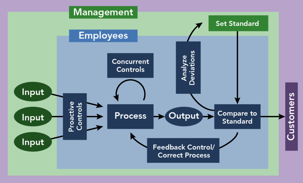
Feedback in closed-loop systems

Feedback is the process of measuring the system output and comparing it to the desired reference signal. The difference between these two values is the error signal, $e(t) = r(t) - y(t)$, where $r(t)$ is the reference and $y(t)$ is the measured output.

Negative feedback is the standard configuration: the control signal acts to reduce the error, driving the system toward the reference. This is what gives closed-loop systems their self-correcting behavior. Positive feedback, by contrast, amplifies the error and is generally destabilizing (though it has niche uses in oscillator circuits and similar applications).

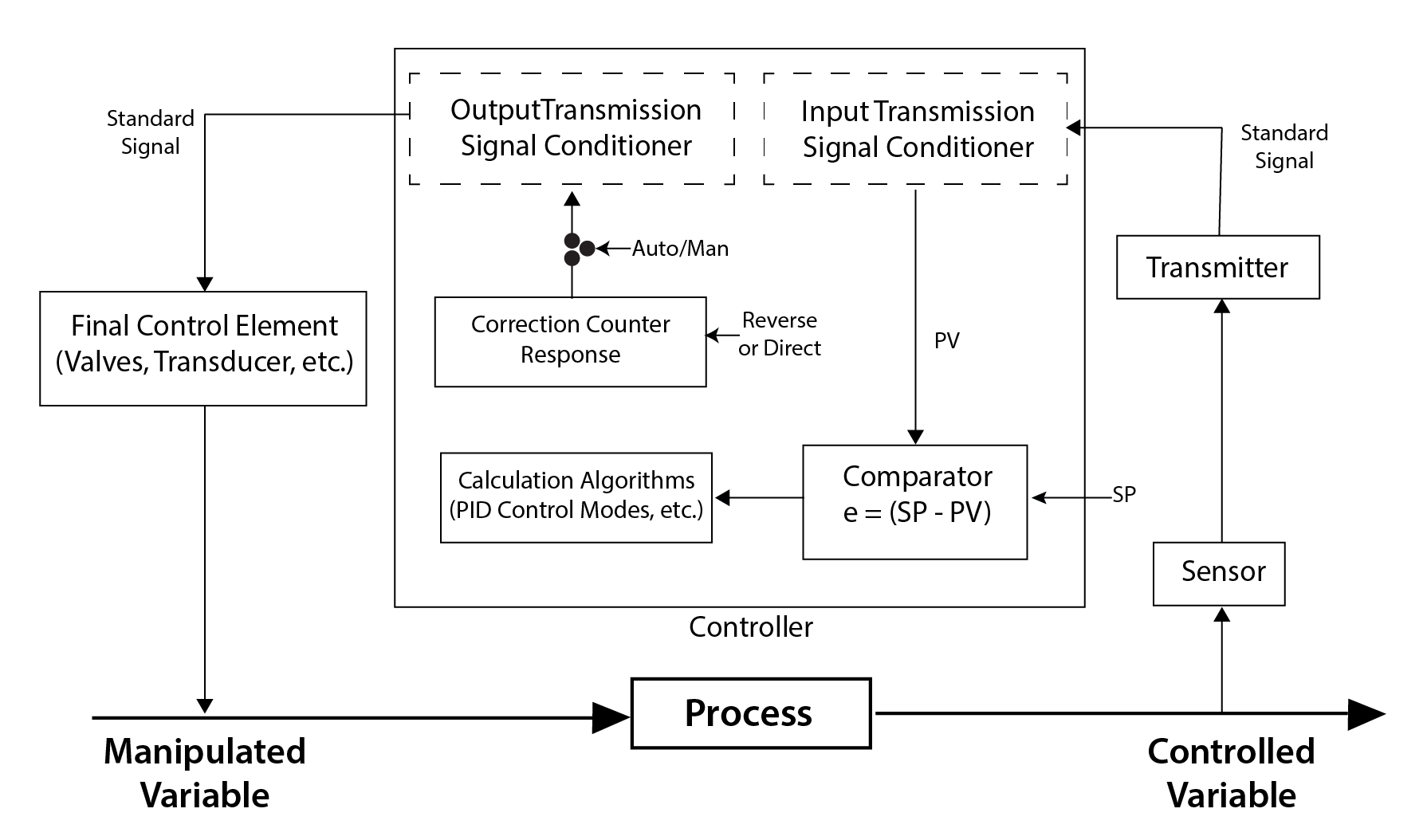
Components of feedback control

A feedback control system has three main components that form a loop: sensors measure the output, the controller computes what action to take, and actuators carry out that action on the physical system.

Role of sensors

• Sensors measure the controlled variable (the system output) and provide that measurement back to the controller
• Accuracy and reliability of the sensor directly limit how well the entire control loop can perform
• Key sensor specifications to consider: measurement range, resolution, response time, and noise characteristics
• Common examples: thermocouples and RTDs for temperature, encoders and potentiometers for position, strain gauges and piezoelectric sensors for pressure

Controller design considerations

The controller is the "brain" of the loop. It takes the error signal, processes it through a control algorithm, and outputs the appropriate control signal to the actuator.

• Controller design involves choosing the control architecture (P, I, D, or a combination) and tuning the gains
• Design goals typically include fast response, minimal overshoot, and low steady-state error
• Modern implementations usually run on digital hardware such as microcontrollers or PLCs, which execute the control algorithm at a fixed sample rate

Actuator selection factors

Actuators convert the controller's electrical signal into a physical action that manipulates the process.

• Selection depends on the required force or torque, speed, precision, and compatibility with the rest of the system
• Common types: electric motors (DC, AC, stepper), hydraulic and pneumatic cylinders, and control valves
• Actuator dynamics (bandwidth, slew rate, dead zone) must be accounted for during control design, since a slow or nonlinear actuator can limit overall system performance

Types of feedback control

The three fundamental control actions are proportional (P), integral (I), and derivative (D). Each addresses a different aspect of the error signal, and they're often combined into a PID controller.

Proportional (P) control

P control produces a control signal directly proportional to the current error:

$u(t) = K_p \, e(t)$

• Higher $K_p$ gives faster response but can cause overshoot and oscillations
• P control alone reduces steady-state error but generally cannot eliminate it entirely. The remaining offset is called droop or proportional offset
• Works well for systems with natural self-regulation, such as flow control or pressure regulation

Integral (I) control

I control produces a signal proportional to the accumulated error over time:

$u(t) = K_i \int_0^t e(\tau) \, d\tau$

• Because it accumulates error, I control will keep adjusting the output until the steady-state error reaches zero
• The downside is integral windup: if the error persists for a long time (e.g., during actuator saturation), the integral term builds up to a large value and causes overshoot when the error finally starts to decrease
• Most useful when zero steady-state error is a hard requirement, such as in precision temperature or position control

Derivative (D) control

D control produces a signal proportional to the rate of change of the error:

$u(t) = K_d \, \frac{de(t)}{dt}$

• Acts as a "predictive" term: if the error is changing rapidly, D control applies a larger corrective action to slow things down before overshoot occurs
• Improves stability and reduces overshoot
• Very sensitive to high-frequency noise in the error signal, since differentiation amplifies noise. In practice, D control is almost always paired with a low-pass filter
• Helpful for systems with slow dynamics or significant time delays

PID control benefits

PID control combines all three actions:

$u(t) = K_p \, e(t) + K_i \int_0^t e(\tau) \, d\tau + K_d \, \frac{de(t)}{dt}$

Each term handles a different job: P provides the main corrective effort, I eliminates steady-state error, and D dampens overshoot and improves stability. The three gains ($K_p$, $K_i$, $K_d$) are tuned to balance these effects for the specific application.

PID controllers are by far the most widely used control algorithm in industry, appearing in HVAC systems, robotics, chemical process control, and countless other domains.

Feedback control performance

Control system performance is evaluated along three axes: stability, transient response, and steady-state error.

Stability analysis techniques

A system is stable if its output converges to the desired value and stays there. An unstable system diverges or oscillates without bound.

• Routh-Hurwitz criterion: an algebraic test that determines stability from the coefficients of the characteristic polynomial, without needing to find the roots
• Nyquist stability criterion: a frequency-domain method that uses the open-loop frequency response to determine closed-loop stability, particularly useful for assessing gain and phase margins
• Root locus: a graphical plot showing how the closed-loop poles move as a parameter (usually gain) varies, giving direct insight into how stability changes with tuning
• Bode plots: frequency-response plots (magnitude and phase vs. frequency) used to read off gain margin and phase margin, which quantify how close the system is to instability

Transient response characteristics

Transient response describes how the system behaves during the transition from one steady state to another, typically evaluated using a step input.

• Rise time ($t_r$): time for the output to go from 10% to 90% of its final value
• Overshoot ($M_p$): the maximum amount the output exceeds its final value, expressed as a percentage
• Settling time ($t_s$): time for the output to stay within a specified tolerance band (commonly ±2% or ±5%) around the final value
• Peak time ($t_p$): time at which the output first reaches its maximum value

These metrics often trade off against each other. For example, reducing rise time by increasing gain tends to increase overshoot.

Steady-state error reduction

Steady-state error ($e_{ss}$) is the persistent difference between the desired and actual output after transients have died out.

• Classified by input type: position error (step input), velocity error (ramp input), and acceleration error (parabolic input)
• Integral control is the most direct way to eliminate steady-state error for step inputs, since the integral term keeps accumulating until the error is zero
• Increasing the system type (the number of pure integrators in the open-loop transfer function) reduces steady-state error for higher-order inputs. A Type 0 system has finite position error; a Type 1 system has zero position error but finite velocity error; and so on

Feedback control design

Control design is the process of building a controller that meets performance specifications while ensuring stability and robustness.

System modeling approaches

Before you can design a controller, you need a mathematical model of the plant (the system being controlled).

• Transfer function models describe the input-output relationship of a linear time-invariant (LTI) system in the Laplace domain, e.g., $G(s) = \frac{Y(s)}{U(s)}$
• State-space models represent the system as a set of first-order differential equations: $\dot{x} = Ax + Bu$, $y = Cx + Du$. These are more general and can handle multi-input multi-output (MIMO) systems naturally
• System identification techniques (frequency response testing, step response fitting, parameter estimation) let you build models from experimental data when first-principles modeling is impractical

Controller tuning methods

Once you have a model, you need to choose the controller gains.

1. Ziegler-Nichols tuning: a classic heuristic method. In the "ultimate gain" version, you increase $K_p$ (with $K_i = 0$, $K_d = 0$) until the system oscillates at a constant amplitude. The gain at that point ($K_u$) and the oscillation period ($T_u$) are plugged into lookup tables to get starting values for $K_p$, $K_i$, and $K_d$.
2. Model-based methods: techniques like pole placement (you specify where you want the closed-loop poles) and LQR (you define cost weights on state error and control effort, and the algorithm computes optimal gains).
3. Iterative/manual tuning: adjust gains one at a time based on observed step responses. A common approach is to set $K_i$ and $K_d$ to zero, increase $K_p$ until you get acceptable speed, then add $K_i$ to remove steady-state error, and finally add $K_d$ to reduce overshoot.

Robustness vs performance trade-offs

Robustness is the system's ability to maintain acceptable stability and performance when the real plant differs from the model, or when unexpected disturbances occur.

• Robust control methods like $H_\infty$ and $\mu$-synthesis explicitly optimize for worst-case uncertainty
• There's a fundamental trade-off: making the controller more robust (conservative) typically reduces nominal performance, and pushing for aggressive performance reduces robustness margins
• The right balance depends on how well you know your plant model and how variable the operating conditions are

Limitations of feedback control

Feedback control is powerful, but it has real constraints that affect what you can achieve in practice.

Sensor noise impact

• Random fluctuations in sensor measurements inject noise into the feedback loop
• Derivative control is especially vulnerable, since differentiating a noisy signal amplifies the high-frequency noise content
• Mitigation strategies: low-pass filtering (moving average, Butterworth filter), Kalman filtering for optimal state estimation, and proper sensor shielding and grounding
• There's a trade-off here too: aggressive filtering reduces noise but adds phase lag, which can hurt stability

Actuator saturation effects

• Every actuator has physical limits (maximum voltage, current, torque, valve opening, etc.). When the control signal exceeds these limits, the actuator saturates and can't deliver what the controller is asking for
• Saturation breaks the linear assumptions of most control designs and can cause instability, especially through integral windup
• Anti-windup techniques address this: integrator clamping (stop accumulating when saturated), conditional integration (pause integration when the actuator is at its limit), and back-calculation (reduce the integral term based on the difference between the commanded and actual actuator output)
• Proper actuator sizing during the design phase helps prevent saturation under normal conditions

Inherent system delays

• Transport delays (fluid flowing through a pipe), communication delays (networked control), and computational delays all introduce phase lag into the loop
• Delays limit the achievable closed-loop bandwidth: the longer the delay relative to the system's time constants, the harder it is to maintain stability at high gains
• Smith predictor: a model-based technique that effectively "removes" a known delay from the feedback loop by predicting what the output will be before the delay elapses
• For uncertain or time-varying delays, robust control methods designed for delay tolerance are more appropriate

Advanced feedback architectures

These architectures extend basic single-loop feedback to handle more complex control challenges.

Cascade control principles

Cascade control uses two (or more) nested feedback loops. The outer loop sets the reference for the inner loop, and the inner loop controls a faster intermediate variable.

• The inner loop rejects disturbances that affect the intermediate variable before they propagate to the primary output
• For cascade control to work well, the inner loop must be significantly faster than the outer loop (typically 3-5x faster)
• Classic example: in a heat exchanger, the outer loop controls the process temperature (slow), while the inner loop controls the coolant flow rate (fast). A disturbance in coolant supply pressure gets corrected by the inner loop before it noticeably affects the temperature
• Tune the inner loop first (with the outer loop open), then tune the outer loop

Feedforward control strategies

Feedforward control measures a disturbance (or knows the reference trajectory in advance) and applies a corrective signal before the disturbance affects the output.

• Unlike feedback, feedforward doesn't wait for an error to appear. This makes it faster at rejecting measurable disturbances
• The catch: feedforward requires an accurate model of how the disturbance affects the output. If the model is wrong, the compensation will be wrong too
• In practice, feedforward is almost always combined with feedback. The feedforward path handles the predictable part of the disturbance, and the feedback loop cleans up whatever the feedforward path misses. This combination is sometimes called two-degree-of-freedom (2-DOF) control

Adaptive control techniques

Adaptive control adjusts controller parameters in real time as the system or its environment changes.

• Model Reference Adaptive Control (MRAC): defines a reference model that represents the desired closed-loop behavior. The controller parameters are adjusted online to minimize the difference between the actual output and the reference model output
• Self-tuning control: estimates the plant parameters in real time (using recursive least squares or similar algorithms) and recalculates the controller gains based on the updated model
• Gain scheduling: the simplest form of adaptive control. Controller gains are pre-computed for several operating points and stored in a lookup table. The system switches between gain sets based on a measurable scheduling variable (e.g., aircraft altitude or speed)
• Adaptive control is valuable when the plant has significant nonlinearities, time-varying parameters, or poorly known dynamics, but it adds complexity and requires careful stability analysis