The Laplace transform converts time-domain functions into a complex frequency domain, turning differential equations into algebraic ones. This is the core technique that makes most of control theory workable. Without it, analyzing even moderately complex systems would require solving differential equations by hand every time.
This guide covers the definition and existence conditions, key properties, common transform pairs, inverse transform techniques, and how Laplace transforms are applied throughout control systems.
Definition of Laplace transforms
The Laplace transform takes a function of time and maps it to a function of the complex variable . The formal definition is:
The integral multiplies by a decaying exponential and sums over all time from 0 to infinity. The result is a function of that encodes the same information as , but in a form where calculus operations become algebra.
Laplace transform vs inverse Laplace transform
- The Laplace transform converts a time-domain function into a complex frequency-domain function
- The inverse Laplace transform converts back into the original time-domain function
These are denoted as:
- Laplace transform:
- Inverse Laplace transform:
The two operations undo each other. You'll typically transform into the -domain to do your analysis or algebra, then invert back to get the time-domain answer.
Laplace transform of derivatives
This is where the real power shows up. Derivatives in time become polynomial expressions in :
The pattern continues for higher-order derivatives: each additional derivative multiplies by another factor of and subtracts initial condition terms. This converts a differential equation into an algebraic equation in , which you can solve with standard algebra.
Laplace transform of integrals
Integration in time becomes division by :
This is useful for solving integro-differential equations (equations that contain both derivatives and integrals of the unknown function) and for analyzing steady-state behavior.
Existence of Laplace transforms
Not every function has a Laplace transform. For to exist, must satisfy two conditions:
- Piecewise continuity: must be piecewise continuous on every finite interval in . A finite number of jump discontinuities is fine.
- Exponential order: There must exist constants and such that for all sufficiently large . This means can't grow faster than some exponential.
These conditions guarantee that the improper integral defining the transform converges. Functions like grow too fast and don't have a Laplace transform, but most signals you'll encounter in control theory (exponentials, sinusoids, polynomials times exponentials) satisfy both conditions.
Properties of Laplace transforms
These properties let you manipulate transforms algebraically instead of re-doing the integral every time. Each property connects a time-domain operation to a simpler frequency-domain operation.
Linearity of Laplace transforms
The Laplace transform is a linear operator:
This means you can break a complex function into simpler pieces, transform each one separately, and add the results. Linearity is the reason Laplace transforms work so well for linear systems.
Frequency shifting in Laplace transforms
Multiplying by an exponential in time shifts the transform in :
If you know the transform of , you get the transform of for free by replacing with . This comes up constantly when dealing with damped oscillations or systems with exponential decay/growth factors.
Time scaling in Laplace transforms
Compressing or stretching time scales the transform:
Here . Speeding up a signal in time (larger ) spreads out its frequency content, and vice versa.
Time shifting in Laplace transforms
Delaying a function by seconds multiplies its transform by an exponential:
The is the unit step function shifted to , which ensures the delayed signal stays zero before the delay kicks in. This property is essential for modeling transport delays and systems where inputs arrive after some lag.
Differentiation in Laplace domain
This repeats the derivative property from earlier, listed here as a formal property:
Differentiation in time corresponds to multiplication by (plus initial condition terms). There's also a dual property: differentiating in the -domain corresponds to multiplication by in time:
Integration in Laplace domain
Integration in time corresponds to division by :
This is particularly handy for computing step responses, since the step response is the integral of the impulse response.
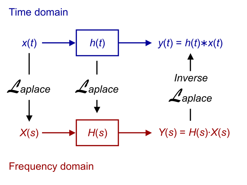
Convolution in Laplace domain
Convolution in time becomes multiplication in the -domain:
where the convolution is defined as .
This is why transfer functions work. The output of an LTI system is the convolution of the input with the impulse response. In the -domain, that convolution becomes simple multiplication: .
Laplace transform tables
Transform tables are your best friend for working with Laplace transforms. Rather than evaluating the integral from scratch, you look up known pairs and use properties to handle variations.
Laplace transforms of common functions
| Time-domain | Laplace transform |
|---|---|
| (impulse) | |
| (unit step) | |
| (ramp) | |
Memorizing at least the first seven of these will save you significant time on exams and homework.
Laplace transforms of periodic functions
For a periodic function with period , you only need the transform of one period. If is the Laplace transform of over the interval (with outside that interval), then:
This works for square waves, sawtooth waves, triangular waves, and any other periodic signal. The denominator accounts for the infinite repetition.
Laplace transforms of special functions
Two special functions appear constantly in control theory:
The Dirac delta function models an idealized impulse (infinite amplitude, zero duration, unit area):
Its transform being simply 1 is why the impulse response of a system equals the inverse transform of the transfer function itself.
The unit ramp function represents a signal that increases linearly from zero:
Step, ramp, and impulse inputs are the three standard test signals used to characterize system behavior.
Applications of Laplace transforms
Laplace transforms for solving ODEs
Laplace transforms provide a systematic method for solving linear ODEs with initial conditions. The procedure is:
- Transform both sides of the ODE using the Laplace transform. Apply the derivative property to handle , , etc., substituting in the given initial conditions.
- Solve for algebraically. Collect all terms involving on one side and solve.
- Invert using partial fractions and the transform table to get .
For example, to solve with and :
- Transforming:
- Simplifying:
- Solving:
- Partial fractions and inversion give the time-domain solution.
This approach handles initial conditions automatically, which is a major advantage over the method of undetermined coefficients.
Laplace transforms for system analysis
In control theory, LTI systems are characterized by their transfer function in the -domain. Taking the Laplace transform of the governing differential equations (with zero initial conditions) yields an algebraic relationship between input and output.
The transfer function captures everything about the system's input-output dynamics: stability, transient behavior, steady-state response, and frequency characteristics. Once you have , you can determine the response to any input by computing and inverting.
Transfer functions in Laplace domain
The transfer function of an LTI system is defined as:
where is the Laplace transform of the output and is the Laplace transform of the input, both with zero initial conditions.
For a system governed by , the transfer function is:
The roots of the numerator are called zeros and the roots of the denominator are called poles. Poles and zeros together determine the system's behavior.

Stability analysis using Laplace transforms
A system's stability is determined by the locations of its transfer function's poles in the complex -plane:
- Stable: All poles have negative real parts (left half-plane). Transients decay to zero.
- Marginally stable: Poles on the imaginary axis with no repeated poles there. Transients neither grow nor decay.
- Unstable: Any pole with a positive real part (right half-plane), or repeated poles on the imaginary axis. Transients grow without bound.
When the transfer function is high-order and factoring the denominator is difficult, the Routh-Hurwitz criterion lets you determine whether all poles are in the left half-plane without actually finding them. Root locus methods provide a graphical way to track pole locations as a design parameter (like controller gain) varies.
Frequency response using Laplace transforms
The frequency response describes how a system responds to sinusoidal inputs at different frequencies. You obtain it by evaluating the transfer function along the imaginary axis:
The result is a complex number for each frequency . Its magnitude tells you the gain (how much the system amplifies or attenuates that frequency), and its angle tells you the phase shift.
Bode plots display magnitude (in dB) and phase (in degrees) versus frequency on a logarithmic scale. These plots reveal bandwidth, resonant peaks, roll-off rate, and gain/phase margins, all of which are critical for controller design.
Inverse Laplace transforms
Getting back from the -domain to the time domain is where you actually extract your answer. Several techniques exist, but partial fraction expansion is by far the most commonly used in practice.
Definition of inverse Laplace transforms
The formal definition is the Bromwich integral:
where is a real constant chosen so the contour of integration lies to the right of all singularities of . You'll rarely evaluate this integral directly. Instead, you'll use the techniques below.
Partial fraction expansion for inverse Laplace
This is the workhorse method. It breaks a complicated rational function into a sum of simple terms you can look up in a table.
Steps:
-
Check degrees. If the numerator degree is greater than or equal to the denominator degree, perform polynomial long division first to get a polynomial plus a proper fraction.
-
Factor the denominator into linear factors and irreducible quadratic factors .
-
Set up partial fractions. For each distinct real pole , write a term . For a repeated pole of multiplicity , write terms . For each irreducible quadratic, write .
-
Solve for coefficients using the Heaviside cover-up method (for distinct real poles) or by multiplying both sides by the denominator and matching coefficients.
-
Invert each term using the transform table.
Residue theorem for inverse Laplace
The residue theorem from complex analysis provides an alternative: the inverse Laplace transform equals the sum of residues of at all poles of .
For a simple (non-repeated) pole at :
For a pole of multiplicity :
This method is most useful when you have high-order repeated poles where partial fractions become tedious.
Bromwich integral for inverse Laplace
The Bromwich integral is the theoretical foundation for the inverse Laplace transform. While you won't typically evaluate it by hand, it's important to know that:
- It guarantees uniqueness: if two continuous functions have the same Laplace transform, they're the same function.
- It can be evaluated using contour integration by closing the contour in the left half-plane and applying the residue theorem, which is how the residue method above is derived.
Numerical methods for inverse Laplace
When is too complex for analytical inversion (non-rational expressions, transcendental functions, or functions known only numerically), numerical methods approximate :
- Gaver-Stehfest algorithm: Approximates using a weighted sum of evaluated at specific real values of . Simple to implement but limited in accuracy for oscillatory functions.
- Talbot algorithm: Deforms the Bromwich contour into a shape that improves numerical convergence. More accurate than Gaver-Stehfest for a wider class of functions.
- Fourier series method (Dubner-Abate): Approximates the inverse transform using a truncated Fourier series expansion.
These are primarily used in computational tools rather than by-hand calculations.
Laplace transforms in control systems
Laplace transforms for modeling systems
Physical systems governed by linear differential equations (mechanical, electrical, thermal, fluid) can all be modeled using transfer functions. The process is:
- Write the governing differential equations from physics (Newton's laws, Kirchhoff's laws, etc.).
- Take the Laplace transform of each equation, assuming zero initial conditions.
- Solve for the transfer function .
Once you have transfer functions for individual components, you can connect them using block diagrams and signal flow graphs. Series connections multiply transfer functions, parallel connections add them, and feedback loops follow the standard formula:
where is the forward path and is the feedback path. This algebraic manipulation of system models is only possible because Laplace transforms convert convolution (the actual physical operation) into multiplication.