2.2 Electrical systems

Electrical systems form the foundation of how control systems interact with the physical world. They handle measurement, signal processing, and actuation, which are the three core tasks any control system needs to perform. This section covers the electrical components used in control systems, how to condition their signals, how to drive actuators with power electronics, and how to build mathematical models of electrical circuits for control design.

Electrical components in control systems

Control systems need electrical components to do three things: measure what's happening in the system (sensors), compute what should happen next (controllers), and make it happen (actuators). Between these stages, signal conditioning circuits clean up sensor data, and power electronics deliver the right amount of energy to actuators.

The main categories of electrical components you'll encounter:

• Sensors for measuring physical quantities (position, velocity, temperature, etc.)
• Actuators for applying control inputs (motors, solenoids, relays)
• Signal conditioning circuits for amplifying, filtering, and digitizing signals
• Power electronics for efficiently controlling power delivery to actuators
• Controllers such as microcontrollers or PLCs (programmable logic controllers)

Sensors for measuring system variables

Sensors provide feedback to the controller about the current state of the system. Without accurate sensing, even the best control algorithm can't do its job. The choice of sensor depends on what variable you're measuring, the required accuracy and resolution, and the operating environment.

Position sensors

Position sensors measure linear or angular displacement relative to a reference point.

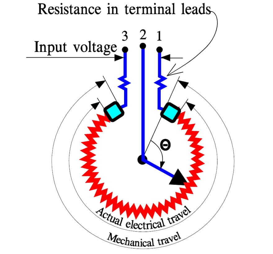
• Potentiometers output a voltage proportional to the position of a sliding contact along a resistive element. Simple and cheap, but subject to wear since there's physical contact.
• Encoders (optical or magnetic) generate digital pulses as a shaft rotates, enabling high-resolution position measurement. An optical encoder with 1024 counts per revolution, for example, gives about 0.35° resolution.
• LVDTs (linear variable differential transformers) use magnetic induction to measure linear displacement without physical contact, making them very durable and suitable for harsh environments.

Velocity sensors

Velocity sensors measure the speed of an object, or equivalently, the rate of change of position.

• You can derive velocity from a position sensor by differentiating the position signal over time, though this amplifies noise.
• Tachometers generate a voltage directly proportional to rotational speed, giving a cleaner velocity signal.
• Doppler effect sensors use the frequency shift of reflected waves (ultrasonic or laser) to measure velocity without contact.

Acceleration sensors

Acceleration sensors measure the rate of change of velocity (the second derivative of position).

• Piezoelectric accelerometers generate an electrical charge proportional to applied acceleration. They're well-suited for vibration and dynamic measurements.
• MEMS accelerometers use the deflection of a microscale cantilever beam to measure acceleration. These are the tiny, inexpensive sensors found in smartphones and automotive airbag systems.

Temperature sensors

• Thermocouples generate a small voltage proportional to the temperature difference between two junctions of dissimilar metals. They cover a wide range (roughly -200°C to 1750°C depending on type) but have lower accuracy.
• RTDs (resistance temperature detectors) change resistance with temperature, typically using a platinum element. They're more accurate than thermocouples but cover a narrower range.
• Thermistors are semiconductor devices with a large resistance change per degree, giving high sensitivity over a limited temperature range.

Pressure sensors

Pressure sensors measure force per unit area exerted by a fluid on a surface.

• Most pressure sensors use a diaphragm or bellows to convert pressure into mechanical displacement, which is then measured by a strain gauge or capacitive element.
• Differential pressure sensors measure the pressure difference between two points and are commonly used for flow measurement (by placing them across an orifice).

Flow sensors

Flow sensors measure the rate of fluid flow through a pipe or channel. Several measurement principles exist:

• Orifice plates and Venturi tubes infer flow rate from the pressure drop across a restriction.
• Turbine flow sensors measure the rotation speed of a small turbine driven by the fluid.
• Thermal mass flow sensors measure how much heat the flowing fluid carries away from a heated element.

Actuators for system control

Actuators convert electrical signals from the controller into physical actions. They're how the control system actually influences the plant.

Electric motors

Electric motors convert electrical energy into rotational mechanical energy.

• DC motors are widely used in control systems because their speed is roughly proportional to applied voltage, making them straightforward to control.
• AC motors (induction and synchronous types) handle high-power applications. Speed control requires varying the input frequency, typically using a variable-frequency drive (VFD).

Solenoids

Solenoids convert electrical energy into linear motion. A coil of wire surrounds a movable iron core (armature). When current flows through the coil, the magnetic field pulls the armature inward. They're used where you need quick, short-stroke linear actuation, such as valves or door locks.

Relays

Relays are electrically operated switches. An electromagnet opens or closes one or more sets of contacts, allowing a low-power control signal to switch a high-power load. They also provide electrical isolation between control circuits and power circuits.

Servomotors

Servomotors allow precise control of angular position. They combine a DC motor, a position sensor (potentiometer or encoder), and a control circuit into one package. The control circuit continuously compares the desired position with the measured position and adjusts the motor to minimize the error. This built-in feedback loop is what makes servos so useful in robotics, CNC machines, and similar applications.

Stepper motors

Stepper motors divide a full rotation into discrete, equal steps. A typical stepper might have 200 steps per revolution (1.8° per step). You control them by sending a specific sequence of pulses to the motor windings, and each pulse advances the motor by one step. This gives precise position control without needing a separate position sensor, which is why they're common in printers, scanners, and 3D printers.

Signal conditioning of sensor outputs

Signal conditioning prepares raw sensor outputs for the controller. Most sensors produce signals that are too weak, too noisy, or in the wrong format (analog vs. digital) to use directly.

Amplification of low-level signals

Many sensors produce millivolt-level outputs. A thermocouple, for instance, might output only about 40 µV per °C.

• Operational amplifiers (op-amps) are the standard building block for signal amplification. The gain is set by the ratio of feedback resistors.
• Instrumentation amplifiers are specialized op-amp circuits designed for accurate, low-noise amplification of small differential signals. They reject common-mode noise, which is critical when sensor leads run through electrically noisy environments.

Filtering of noise

Sensor outputs often contain unwanted noise that must be removed before the signal reaches the controller.

• Low-pass filters remove high-frequency noise such as electromagnetic interference (EMI) or 50/60 Hz power line pickup.
• High-pass filters remove low-frequency drift or DC offset voltages.
• Band-pass filters pass only a specific frequency range while attenuating everything else.
• Active filters use op-amps to achieve sharper roll-off characteristics and adjustable cutoff frequencies compared to passive RC filters.

Analog-to-digital conversion

Modern controllers operate digitally, so analog sensor signals must be converted using an analog-to-digital converter (ADC).

• The ADC samples the continuous signal at discrete time intervals and quantizes the amplitude into a finite number of levels.
• Resolution (number of bits) determines the smallest detectable change. A 12-bit ADC dividing a 0–5 V range gives about 1.22 mV per step.
• Sampling rate must satisfy the Nyquist theorem: sample at least twice the highest frequency component in the signal, or you'll get aliasing (false low-frequency artifacts).
• Multiplexers allow multiple analog channels to share a single ADC by connecting them sequentially, reducing hardware cost.

Power electronics for actuator control

Power electronics efficiently control the flow of electrical power to actuators. Rather than wasting energy as heat (like a variable resistor would), power electronic circuits use semiconductor switches to chop and regulate power.

Transistors vs thyristors

• Transistors (MOSFETs and IGBTs) can be fully turned on or off by a gate signal, making them ideal for fast switching and PWM control. MOSFETs dominate at lower power levels; IGBTs handle medium to high power.
• Thyristors (SCRs and triacs) are used in very high-power applications. Once triggered on, a thyristor latches and stays on until the current drops below a holding threshold. This makes them simpler for AC power control but less flexible than transistors.

Pulse-width modulation (PWM)

PWM controls the average voltage or current delivered to an actuator by rapidly switching power on and off.

• The duty cycle (ratio of on-time to total period) determines the effective output. A 75% duty cycle on a 12 V supply delivers an average of 9 V to the load.
• PWM is far more efficient than linear regulation because the switching device is either fully on (low resistance, low loss) or fully off (no current, no loss).
• The PWM frequency must be high enough to smooth out current ripple in the actuator, but not so high that switching losses become significant. For DC motors, frequencies of 5–20 kHz are typical.

H-bridges for motor control

An H-bridge is a circuit of four switches arranged in an "H" pattern around a DC motor. By controlling which pair of switches is closed, you can:

• Drive current forward through the motor (forward rotation)
• Drive current backward through the motor (reverse rotation)
• Short both terminals together (dynamic braking)

The switches are typically controlled with PWM signals to regulate speed in addition to direction.

Protection circuits

Power electronics need protection against faults:

• Overcurrent protection: Fuses or electronic current limiters prevent excessive current from damaging switches or the actuator.
• Overvoltage protection: Transient voltage suppressors or snubber circuits clamp voltage spikes caused by inductive loads (motors, solenoids) during switching.
• Thermal protection: Temperature sensors trigger shutdown if power devices overheat.
• Isolation: Optocouplers or transformers provide electrical isolation between the low-voltage control stage and the high-voltage power stage, protecting the controller from dangerous voltages and noise.

Electrical system modeling

Modeling electrical systems means building mathematical representations that predict how circuits behave. These models let you simulate responses, design controllers, and verify stability before building hardware.

Kirchhoff's laws

These two laws are the starting point for writing circuit equations:

• Kirchhoff's Current Law (KCL): The sum of all currents entering a node equals the sum of all currents leaving that node. This comes from conservation of charge.
• Kirchhoff's Voltage Law (KVL): The sum of all voltages around any closed loop in a circuit equals zero. This comes from conservation of energy.

You use KCL and KVL together to derive the differential equations that describe a circuit's behavior.

Impedance and admittance

Impedance ($Z$) generalizes resistance to AC circuits by accounting for both resistance and reactance:

• Resistors have impedance $Z_R = R$ (purely real)
• Inductors have impedance $Z_L = sL$ (in the Laplace domain) or $Z_L = j\omega L$ (in the frequency domain)
• Capacitors have impedance $Z_C = \frac{1}{sC}$ or $Z_C = \frac{1}{j\omega C}$

Impedance is a complex quantity: the real part is resistance, and the imaginary part is reactance. Admittance ($Y = \frac{1}{Z}$) is the reciprocal and represents how easily current flows.

Using impedance, you can analyze AC circuits with the same series/parallel rules you'd use for resistors in DC circuits.

Transfer functions of electrical components

Transfer functions describe the input-output relationship of a system in the Laplace domain. You obtain them by applying the Laplace transform to the circuit's differential equations (assuming zero initial conditions).

The basic component relationships in the Laplace domain:

• Resistor: $V(s) = R \cdot I(s)$
• Inductor: $V(s) = sL \cdot I(s)$
• Capacitor: $V(s) = \frac{1}{sC} \cdot I(s)$

To find the transfer function of a circuit:

1. Label all voltages and currents in the Laplace domain.
2. Write KVL and KCL equations using impedances.
3. Solve algebraically for the ratio of output to input: $H(s) = \frac{Y(s)}{X(s)}$.

Transfer functions of individual components can be combined using series and parallel connection rules to build up the overall system transfer function.

State-space representation

State-space representation models a system as a set of first-order differential equations. It's especially useful for multi-input, multi-output (MIMO) systems where transfer functions become unwieldy.

The general form:

$\dot{x} = Ax + Bu$

$y = Cx + Du$

where:

• $x$ is the state vector (the minimal set of variables that fully describes the system at any instant)
• $u$ is the input vector
• $y$ is the output vector
• $A$ is the system matrix, $B$ is the input matrix, $C$ is the output matrix, $D$ is the feedthrough matrix

For electrical circuits, the state variables are typically capacitor voltages and inductor currents, since these are the energy-storing elements whose values can't change instantaneously.

State-space models enable analysis of stability, controllability, and observability using linear algebra techniques.

Electrical system analysis

Once you have a model, you need tools to evaluate how the system behaves. The main analysis approaches are frequency response, stability analysis, pole-zero analysis, and transient/steady-state response characterization.

Frequency response

Frequency response describes how a system's output amplitude and phase shift change as you sweep a sinusoidal input across different frequencies.

• Bode plots are the standard visualization: a magnitude plot (in dB) and a phase plot (in degrees) versus frequency on a log scale.
• The magnitude plot shows the system's gain at each frequency. The phase plot shows how much the output lags or leads the input.
• Frequency response analysis reveals resonant frequencies, bandwidth (the range of frequencies the system responds to effectively), and stability margins.

Stability analysis using Nyquist and Bode plots

A system is stable if its output remains bounded for any bounded input.

Nyquist criterion: Plot the open-loop transfer function $G(j\omega)H(j\omega)$ as a polar curve. The closed-loop system is stable if the number of counterclockwise encirclements of the point $-1 + j0$ equals the number of unstable open-loop poles.

Bode plot stability margins:

• Gain margin: How much you can increase the loop gain before the system goes unstable. Measured at the frequency where phase equals -180°.
• Phase margin: How much additional phase lag the system can tolerate before instability. Measured at the frequency where gain equals 0 dB (the gain crossover frequency).

Poles and zeros

Poles and zeros are the roots of the denominator and numerator polynomials of the transfer function $H(s)$, respectively.

• Poles determine the system's natural modes of response (natural frequencies and damping).
• Zeros determine frequencies where the system's response is suppressed.

Their location in the complex $s$-plane tells you about stability and dynamics:

• Poles in the left-half plane (LHP): stable (decaying) modes
• Poles in the right-half plane (RHP): unstable (growing) modes
• Poles on the imaginary axis: sustained oscillations (marginally stable)
• Poles close to the imaginary axis: lightly damped, oscillatory response
• RHP zeros can cause non-minimum phase behavior (initial response in the wrong direction before correcting)

Transient response vs steady-state response

Transient response is the system's behavior right after an input is applied. Key metrics:

• Rise time: Time to go from 10% to 90% of the final value
• Overshoot: Maximum deviation beyond the final value, expressed as a percentage
• Settling time: Time to stay within a specified tolerance band (typically ±2%) of the final value
• Peak time: Time at which the maximum overshoot occurs

Steady-state response is the system's behavior long after transients have died out. The key metric is steady-state error, which is the difference between the desired and actual output. The system type (number of integrators in the open-loop transfer function) determines which input types (step, ramp, parabolic) the system can track with zero steady-state error.

Control design often involves trading off between transient performance (fast rise time, low overshoot) and steady-state accuracy (small or zero steady-state error).

Electrical system design considerations

Designing electrical systems for control applications requires balancing multiple factors: power supply requirements, component ratings, thermal management, electromagnetic compatibility, and safety. These practical concerns determine whether a theoretically sound design actually works reliably in the real world.